Heapsort (Heap Sort) – Algorithm, Java Code, Time Complexity

With Heapsort, most Java developers first think of the Java heap. This article will show you that Heapsort is something completely different – and how Heapsort works precisely.

You’ll find out in detail:

• What is a Heap?
• How does the Heapsort algorithm work?
• What does the Heapsort source code look like?
• How to determine Heapsort’s time complexity?
• What is Bottom-Up Heapsort, and what are its advantages?
• How does Heapsort compare to Quicksort and Merge Sort?

What is a Heap?

A “heap” is a complete binary tree in which each node is either greater than or equal to its children (“max heap”) – or less than or equal to its children (“min heap”).

Complete means: All levels of the tree are full; only the bottom level may be missing nodes on the right.

Here is a simple example of a “max heap”:

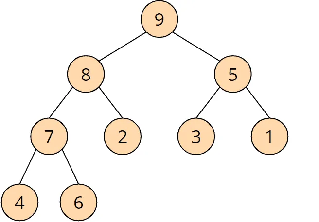
The 9 is greater than the 8 and the 5; the 8 is greater than the 7 and the 2; etc.

A heap is projected onto an array by transferring its elements line by line from top left to bottom right into the array:

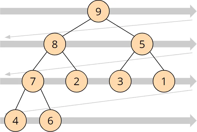
The heap shown above looks like this as an array:

Because the tree is complete, the array needs no references between the nodes. The position of an element determines where its children and its parent are.

The children of the element at index i are at indexes 2i + 1 and 2i + 2, its parent at index (i − 1) / 2 (rounded down). The following picture shows this for the 8 at index 1:

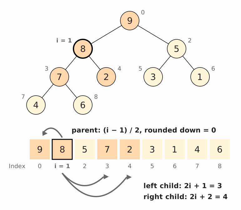
The last parent node is the parent of the last element. It is at index n / 2 − 1 (with n / 2 rounded down) – for the nine elements of the example, at index 3, which holds the 7.

In a “max heap”, the largest element is always at the top – in the array form, it is, therefore, on the far left. The following section explains how to use this characteristic for sorting.

Heapsort Algorithm

The heapsort algorithm consists of two phases: In the first phase, the array to be sorted is converted into a max heap. And in the second phase, the largest element (i.e., the one at the tree root) is removed, and a new max heap is created from the remaining elements.

The following sections explain the two phases in detail using an example:

Phase 1: Creating the Heap

The array to be sorted must first be converted into a heap. For this purpose, no new data structure is created, but the numbers are rearranged within the array so that the heap structure described above is created.

In the following example, I explain how exactly this is done using the number sequence known from the previous parts of the article series: [3, 7, 1, 8, 2, 5, 9, 4, 6].

We “project” these numbers onto a binary tree, as described above. The binary tree is not a separate data structure, but only a thought construct – in the computer’s memory, the elements are located exclusively in the array.

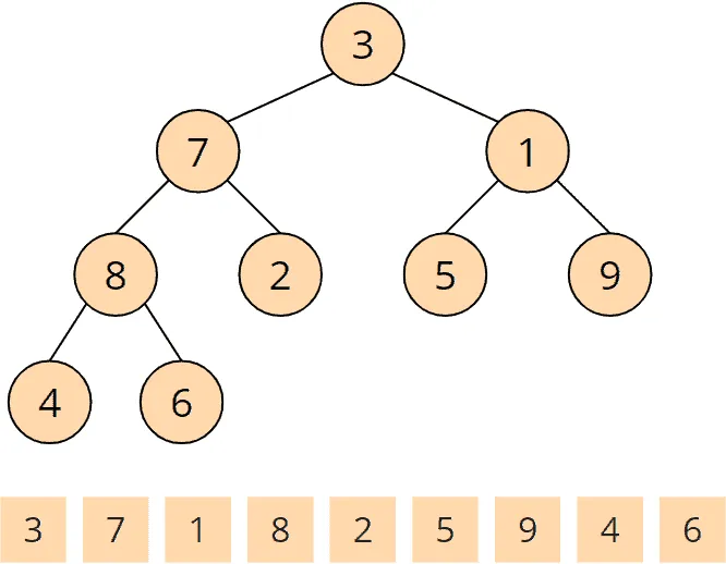
This tree does not yet represent a max heap. The definition of a max heap is that parents are always greater than or equal to their children.

To create a max heap, we now visit all parent nodes – backward from the last one to the first – and make sure that the heap condition for the respective node and the nodes below it is fulfilled. We do this using the so-called heapify() method.

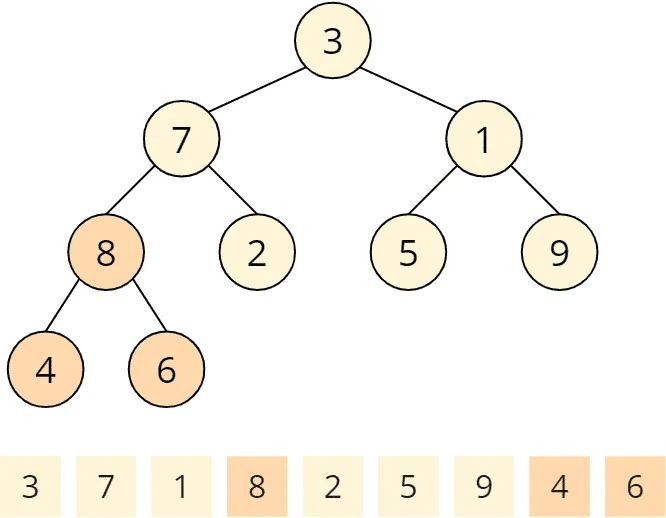
Invocation No. 1 of the Heapify Method

The heapify() method is called first for the last parent node. Parent nodes are 3, 7, 1, and 8. The last parent node is 8. The heapify() method checks if the children are smaller than the parent node. 4 and 6 are smaller than 8, so at this parent node, the heap condition is fulfilled, and the heapify() method is finished.

Invocation No. 2 of the Heapify Method

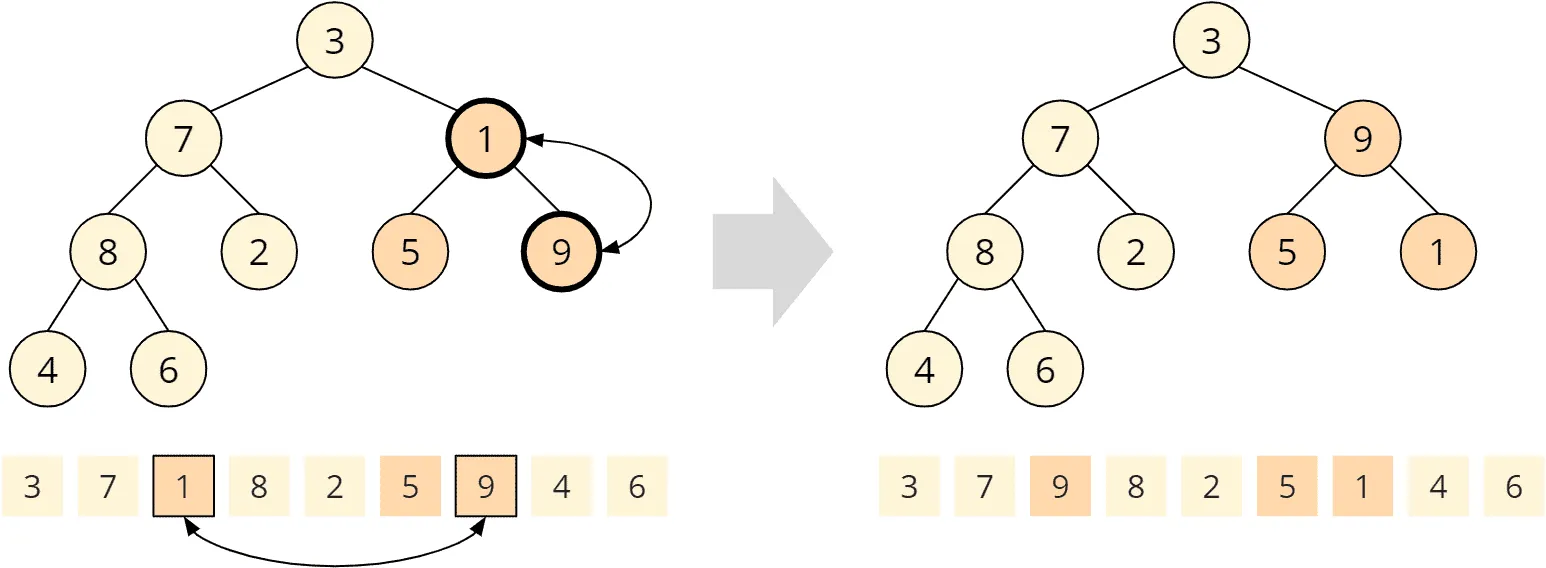
Second, heapify() is called for the penultimate parent node: the 1. Its children 5 and 9 are both greater than 1, so the heap condition is violated. To restore the heap condition, we now swap the larger child with the parent node, i.e., the 9 with the 1. The heapify() method is now finished again.

Invocation No. 3 of the Heapify Method

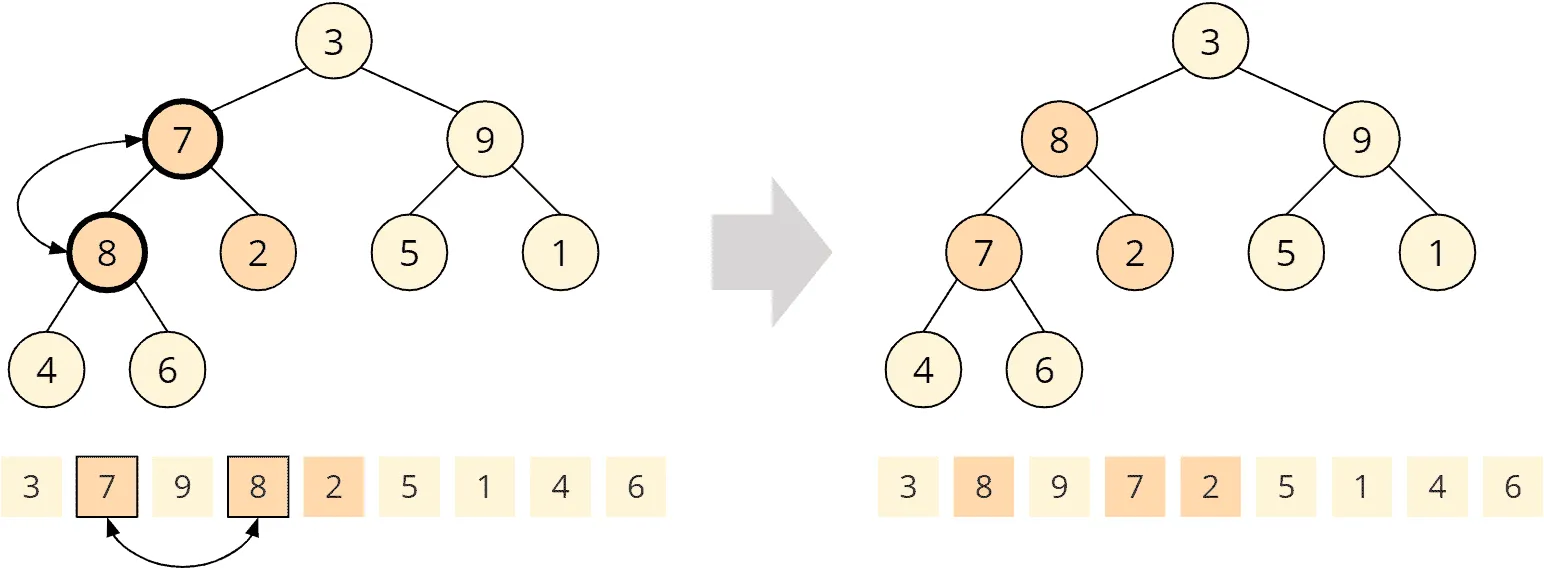
Now heapify() is called on the 7. Child nodes are 8 and 2; only the 8 is larger than the parent node. So we exchange the 7 with the 8:

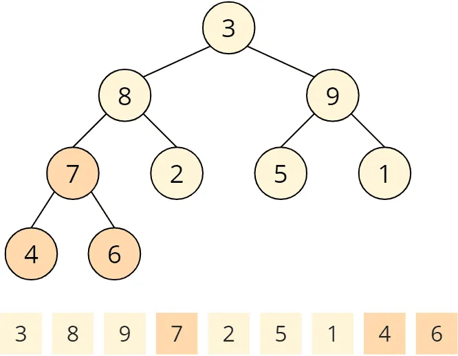
Since the child node we just swapped has two children itself, the heapify() method must now check if the heap condition for this child node is still valid. In this case, the 7 is greater than 4 and 6; the heap condition is fulfilled, and the heapify() method is finished.

Invocation No. 4 of the Heapify Method

Now we have arrived at the root node with element 3. Both child nodes, 8 and 9, are larger; the 9 is the larger child and is, therefore, swapped with the parent node:

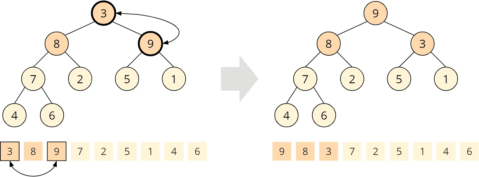
Again, the swapped child node has children itself, so we need to check the heap condition on this child node. The 5 is greater than the 3, i.e., the heap condition is not fulfilled. It must be restored by swapping the 5 and the 3:

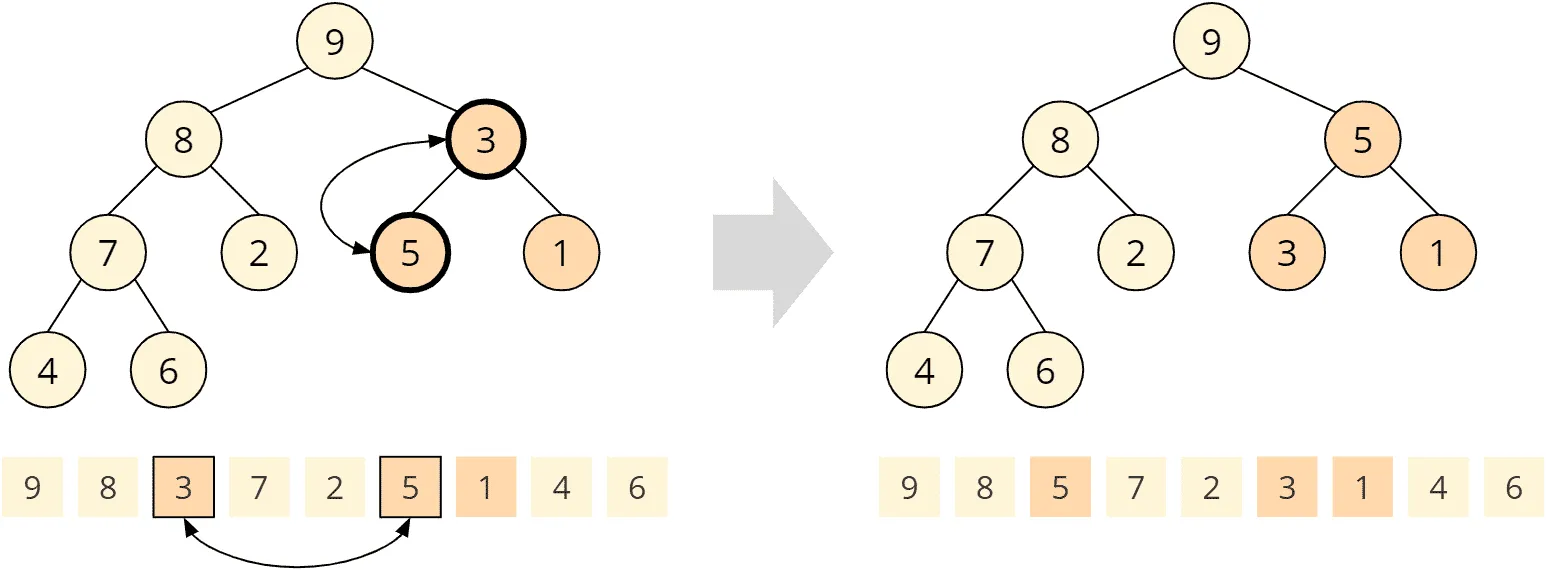
The fourth and last call of the heapify() method has finished. A max heap has been created:

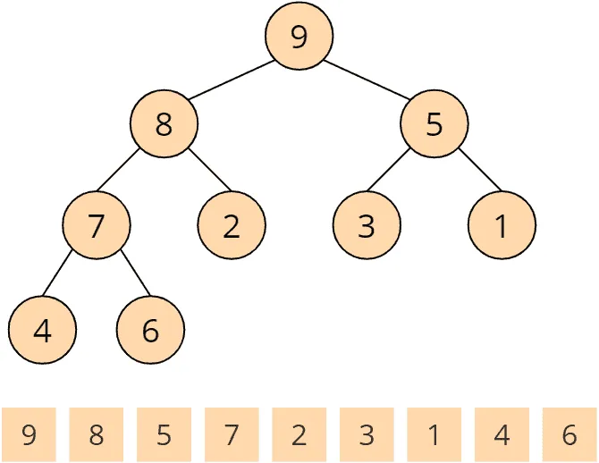
Which brings us to phase two of the heapsort algorithm.

Phase 2: Sorting the Array

In phase 2, we take advantage of the fact that the largest element of the max heap is always at its root (in the array: on the far left).

Phase 2, Step 1: Swapping the Root and Last Elements

The root element (the 9) is now swapped with the last element (the 6) so that the 9 is at its final position at the end of the array (marked blue in the array). We also remove this element from the tree (displayed in grey):

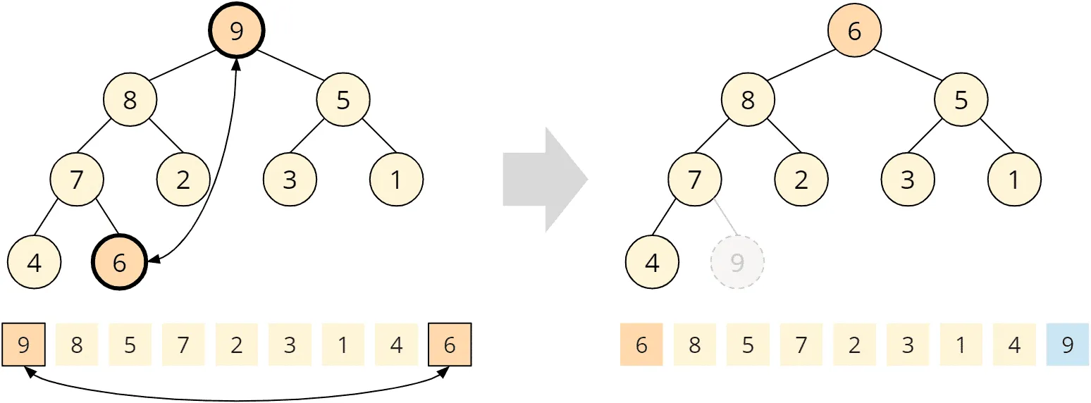
After we’ve placed the 6 at the root of the tree, it is no longer a max heap. Therefore, in the next step, we will “repair” the heap.

Phase 2, Step 2: Restoring the Heap Condition

To restore the heap condition, we call the heapify() method known from phase 1 on the root node. This means we compare the 6 with its children, 8 and 5; the 8 is bigger, so we swap it with the 6:

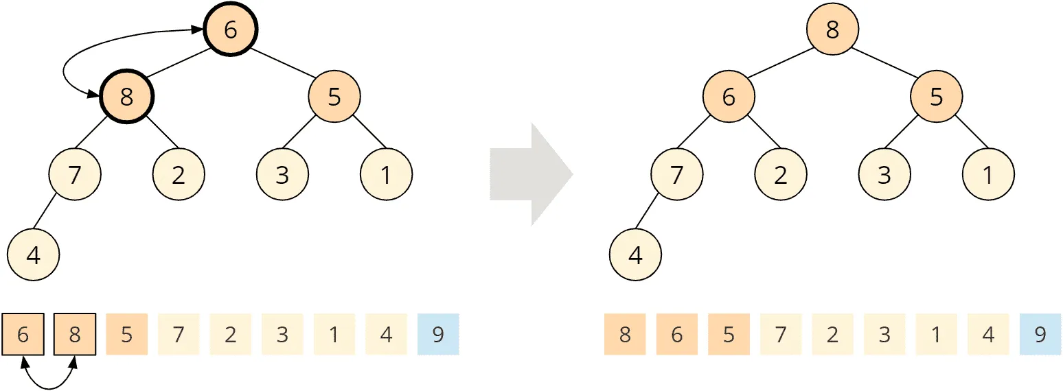
The swapped child node has, in turn, two children, the 7 and the 2. The 7 is larger than the 6, and we swap these two elements as well:

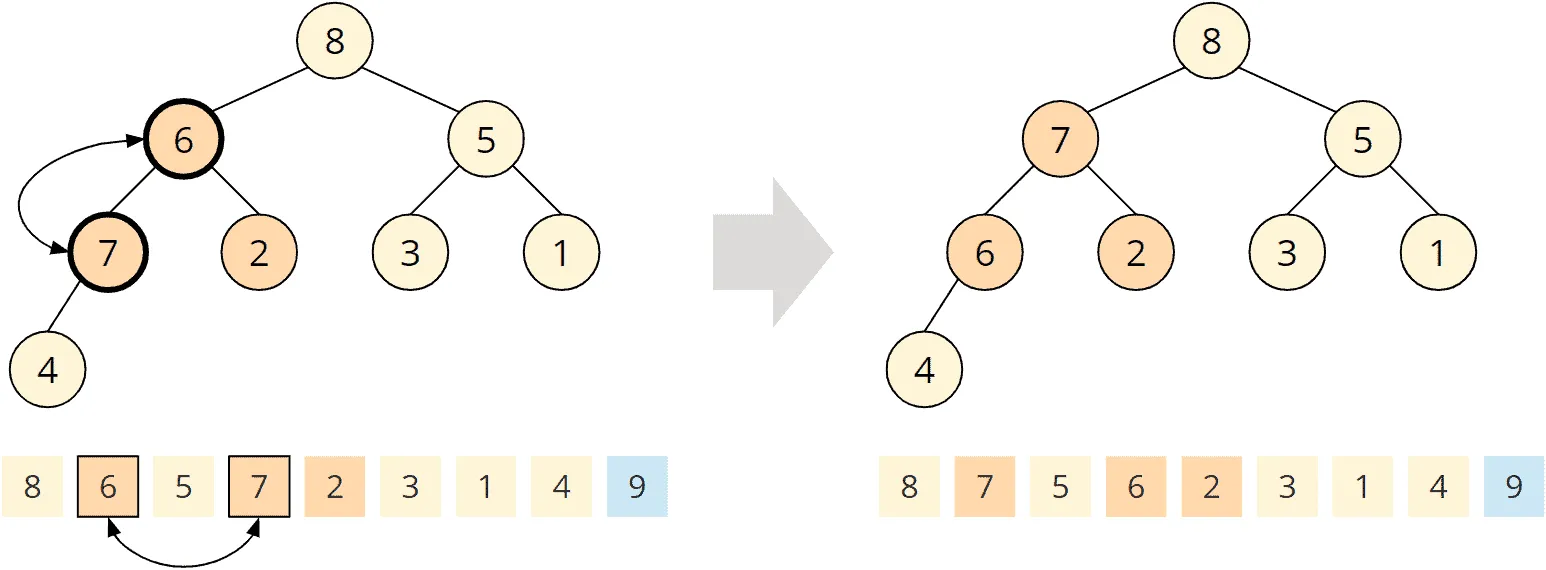
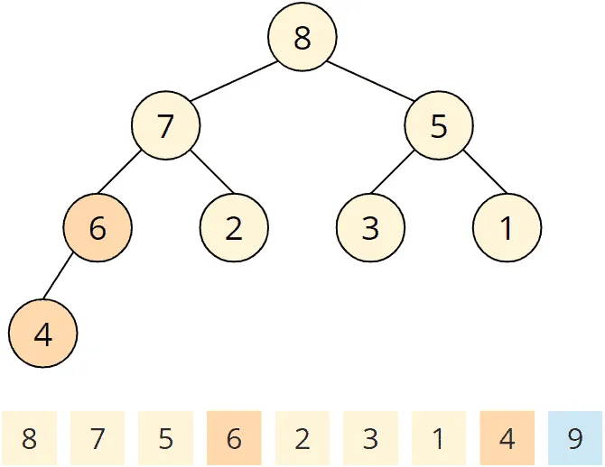
The exchanged child node also has a child, the 4. The 6 is greater than the 4, so the heap condition is fulfilled at this node. The heapify() method is finished, and we have a max heap again:

Repeating the Steps

The largest number of the remaining array, 8, is now in the first position. We swap it with the last element of the tree. Since we have shortened the tree by one element, the last element of the tree is on the second-to-last field of the array:

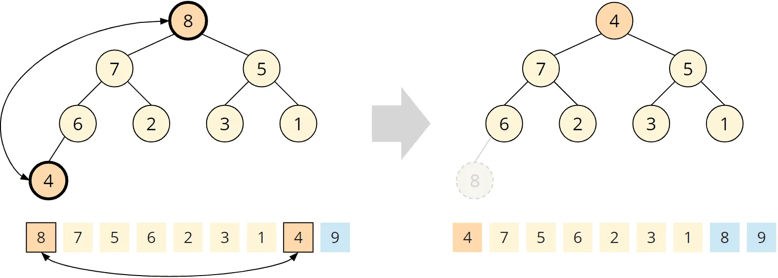
Now, the last two fields of the array are sorted.

At the root, the heap condition is violated again. We repair the tree by calling heapify() on the root element (the following picture shows all heapify steps at once).

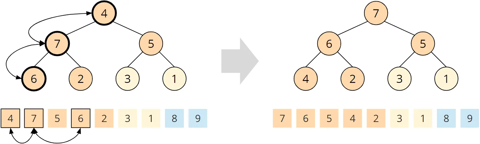
We repeat the process until there is only one element left in the tree:

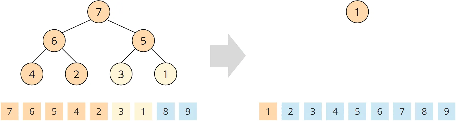
This element is the smallest and remains at the beginning of the array. The algorithm is finished, the array is sorted:

Heapsort Java Code Example

In this section, you’ll find the source code of Heapsort.

The sort() method first calls buildHeap() to initially build the heap.

In the following loop, the variable swapToPos iterates backward from the end of the array to its second field. In the loop body, the first element is swapped with the one at the swapToPos position, and then the heapify() method is called on the subarray up to, but not including, position swapToPos:

public class Heapsort {

  public void sort(int[] elements) {
    buildHeap(elements);

    for (int swapToPos = elements.length - 1; swapToPos > 0; swapToPos--) {
      // Move root to end
      ArrayUtils.swap(elements, 0, swapToPos);

      // Fix remaining heap
      heapify(elements, swapToPos, 0);
    }
  }

  [...]
}

The buildHeap() method calls heapify() for each parent node, starting with the last one, and passes to this method the array, the length of the subarray representing the heap, and the position of the parent node where heapify() should start:

void buildHeap(int[] elements) {
  // "Find" the last parent node
  int lastParentNode = elements.length / 2 - 1;

  // Now heapify it from here on backwards
  for (int i = lastParentNode; i >= 0; i--) {
    heapify(elements, elements.length, i);
  }
}

The heapify() method checks whether a child node is larger than the parent node. If this is the case, the parent element is swapped with the larger child element, and the process is repeated on the child node.

void heapify(int[] heap, int length, int parentPos) {
  while (true) {
    int leftChildPos = parentPos * 2 + 1;
    int rightChildPos = parentPos * 2 + 2;

    // Find the largest element
    int largestPos = parentPos;
    if (leftChildPos < length && heap[leftChildPos] > heap[largestPos]) {
      largestPos = leftChildPos;
    }
    if (rightChildPos < length && heap[rightChildPos] > heap[largestPos]) {
      largestPos = rightChildPos;
    }

    // largestPos is now either parentPos, leftChildPos or rightChildPos.
    // If it's the parent, we're done
    if (largestPos == parentPos) {
      break;
    }

    // If it's not the parent, then switch!
    ArrayUtils.swap(heap, parentPos, largestPos);

    // ... and fix again starting at the child we moved the parent to
    parentPos = largestPos;
  }
}

The loop in heapify() could also be written recursively – but then the call stack would need O(log n) additional memory.

You can find the source code in the Heapsort class in the GitHub repository. It is slightly different from the class printed here: The class in the repository implements the SortAlgorithm interface to be interchangeable within the test framework.

Heapsort Time Complexity

Click on the following link for an introduction to “time complexity” and “O notation” (with examples and diagrams).

Time Complexity of the heapify() Method

Let’s start with the heapify() method since we also need it for the heap’s initial build.

In the heapify() method, we walk through the tree from top to bottom. The height of a heap – i.e., a complete binary tree – of size n is log₂ n (rounded down, the root not being counted), i.e., if the number of elements doubles, the tree becomes only one level deeper:

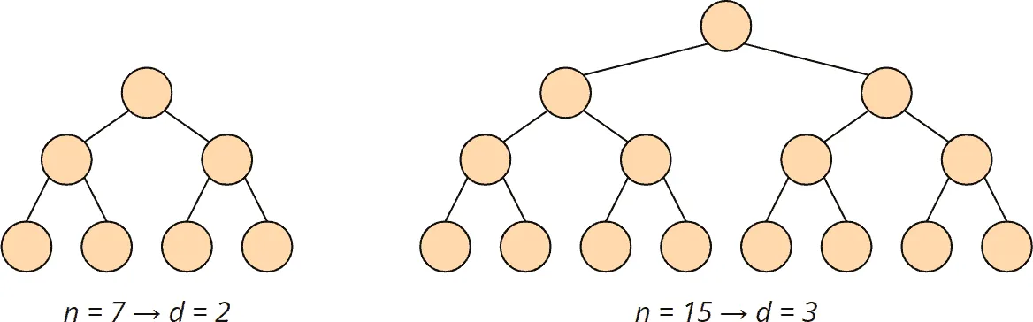
The complexity for the heapify() method is accordingly O(log n).

Time Complexity of the buildHeap() Method

To initially build the heap, the heapify() method is called for each parent node – backward, starting with the last node and ending at the tree root.

A heap of size n has n/2 (rounded down) parent nodes:

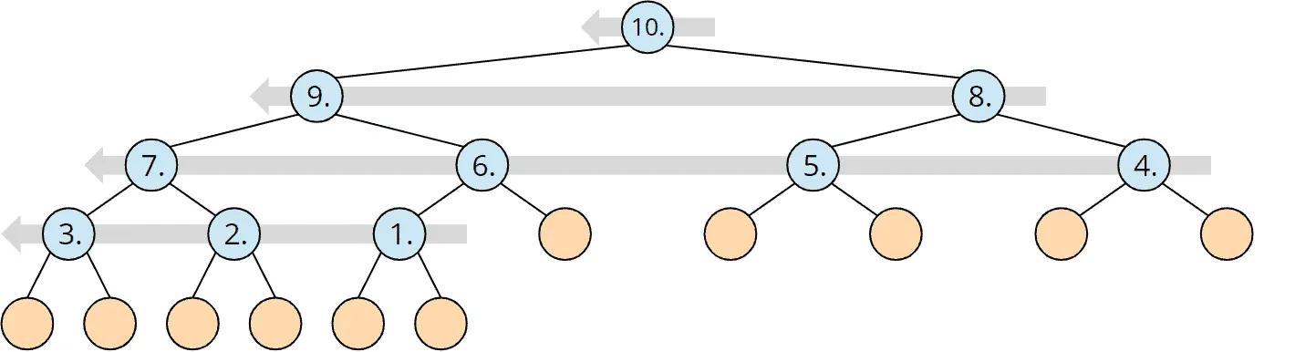
Since the complexity of the heapify() method is O(log n) as shown above, the complexity for the buildHeap() method is, therefore, maximum* O(n log n).

* In the section after the next one, I will show that the time complexity of the buildHeap() method is actually O(n). Since this does not change the overall time complexity, it is not mandatory to perform this in-depth analysis.

Total Time Complexity of Heapsort

In phase 2, the heapify() method is called (n − 1) times. So the total complexity for repairing the heap is also O(n log n).

Both sub-algorithms, therefore, have the same time complexity. Hence:

The time complexity of Heapsort is: O(n log n).

This holds for the average and the worst case. It gets faster when all elements are equal: Then heapify() never finds a larger child and stops every time after comparing the two children, without swapping – in this case, Heapsort sorts in O(n).

Time Complexity for Building the Heap – In-Depth Analysis

This section is very mathematical and not necessary for determining the time complexity of the overall algorithm (which we have already completed). You could, therefore, skip this section.

We have seen above that the buildHeap() method calls heapify() for each parent node. What we have not considered so far is that the depth of the subtrees, on which heapify() is called, varies. The following graphic illustrates this (d stands for the depth of the subtrees):

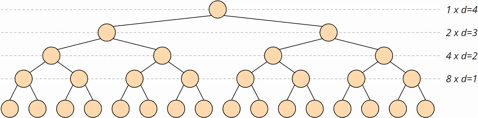
The heapify() method is called at most for n/4 trees of depth 1, for n/8 trees of depth 2, for n/16 trees of depth 3, etc.

The maximum number of swap operations in the heapify() method is equal to the depth of the subtree on which it is called.

The maximum number of swap operations S_max is therefore:

S_max = n/4 · 1 + n/8 · 2 + n/16 · 3 + n/32 · 4 + ...

If we multiply both sides of the term by 2, we get:

2 · S_max = n/2 · 1 + n/4 · 2 + n/8 · 3 + n/16 · 4 + ...

Let us place both terms on top of each other:

2 · Smax =	n/2 · 1 +	n/4 · 2 + n/8 · 3 + n/16 · 4 + ...
Smax =		n/4 · 1 + n/8 · 2 + n/16 · 3 + n/32 · 4 + ...

Both terms contain n/4, n/8, n/16 etc. with a factor differing by the constant 1. If we subtract the terms, we get:

2 · S_max − S_max = n/2 · 1 + n/4 · (2 − 1) + n/8 · (3 − 2) + n/16 · (4 − 3) + ...

This can be simplified to:

S_max = n/2 + n/4 + n/8 + n/16 + ...

Or:

S_max = n · (1/2 + 1/4 + 1/8 + 1/16 + ...)

The term 1/2 + 1/4 + 1/8 + 1/16 + ... approaches 1, as shown in the following diagram:

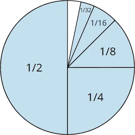
Thus the formula can finally be simplified to:

S_max ≤ n

We have thus shown that the effort required to build the heap is linear, i.e., the time complexity is O(n).

However, the total complexity of O(n log n) mentioned above does not change due to the lower complexity class of a partial algorithm.

Runtime of the Java Heapsort Example

The UltimateTest class can be used to determine the runtime of different sorting algorithms for different input sizes.

The following table shows the medians of the runtimes for sorting randomly arranged, as well as ascending and descending presorted elements (this is only an excerpt for the sake of clarity):

n	unsorted	ascending	descending
...	...	...	...
2,097,152	172.6 ms	80.3 ms	85.7 ms
4,194,304	381.4 ms	165.3 ms	177.0 ms
8,388,608	893.2 ms	341.5 ms	364.0 ms
16,777,216	2,298.4 ms	700.0 ms	750.2 ms
33,554,432	5,663.5 ms	1,434.7 ms	1,537.5 ms
67,108,864	13,005.5 ms	2,962.3 ms	3,158.8 ms

Here are the measurements as a diagram:

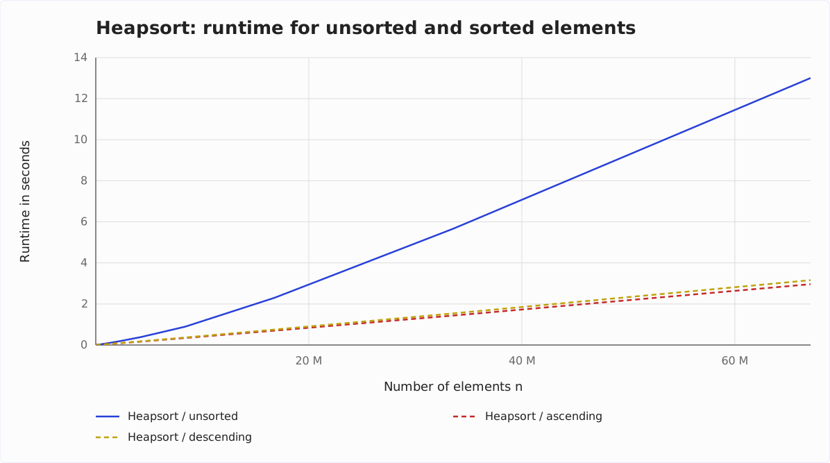
You can see clearly:

• When doubling the input quantity, sorting presorted elements takes a little more than twice as long (factor 2.05 to 2.07 in the table); this corresponds to the expected quasilinear runtime O(n log n). For unsorted elements, the factor rises to up to 2.6.
• For presorted input data, Heapsort is 2.1 to 4.4 times as fast as for unsorted data (descending order: 2.0 to 4.1 times) – the larger the array, the greater the difference.
• Input data sorted in descending order takes about 7% longer than input data sorted in ascending order.

Why Is Heapsort Faster for Presorted Input Data?

To address this question, I use the program CountOperations to count the compare, read, and write operations of Heapsort in both phases – for unsorted as well as ascending and descending sorted data.

You can find the result in the file CountOperations_Heapsort.log. The results of the test are:

• If the input data is sorted in descending order, there are only about half as many comparisons in phase 1 as there are for unsorted or ascending data; there are also no swap operations. This is because a descending sorted array already corresponds to a max heap.
• Input data sorted in ascending order correspond to a min heap. The tree must be completely reversed in the buildHeap() phase, so in this case, we have about a third more swap operations than with randomly arranged data, in which the heap condition is already fulfilled on some subtrees.
• In phase 2, the number of operations differs only slightly.

Then how can we explain that Heapsort is so much faster for both ascending and descending presorted input data?

The obvious explanation is the so-called branch prediction.

With presorted input data, the comparison operations always lead to the same result. If the branch prediction now assumes that the comparisons will also lead to the same result in the future, the CPU’s instruction pipelines can be fully utilized.

With unsorted input data, however, no reliable statement can be made about future comparison results. As a result, the instruction pipeline must often be flushed and refilled.

Bottom-Up Heapsort

Bottom-Up Heapsort is a variant in which the heapify() method makes do with fewer comparisons through smart optimization. This is advantageous if, for example, we don’t compare int primitives, but objects with a time-consuming compareTo() method.

In the regular heapify(), we perform two comparisons on each node from top to bottom to find the largest of three elements:

1. Parent node with left child
2. The larger node from the first comparison with the second child

Bottom-Up Heapsort Algorithm

Bottom-Up Heapsort, on the other hand, only compares the two children and follows the larger child to the end of the tree (“top-down”). From there, the algorithm goes back towards the tree root (“bottom-up”) and searches for the first element that is not smaller than the root. From this position, all elements are moved one position towards the root, and the root element is placed in the field that has become free.

The following example should make it easier to understand.

Bottom-Up Heapsort Example

In the following example, we compare the 9 and 4, then the children of the 9 – the 8 and the 6, and finally the children of the 8 – the 7 and the 3:

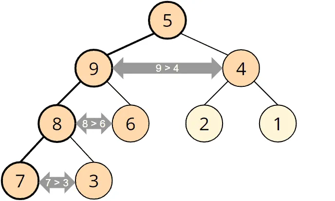
In this way, we reach the 7 and compare it with the tree root, the 5:

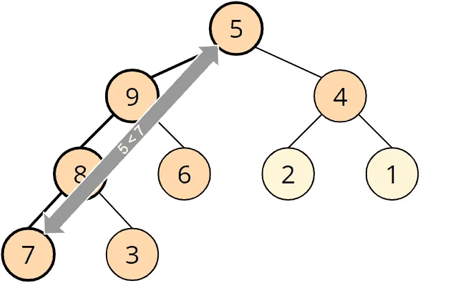
The 5 is smaller than the 7, which means that the root element must be passed all the way down:

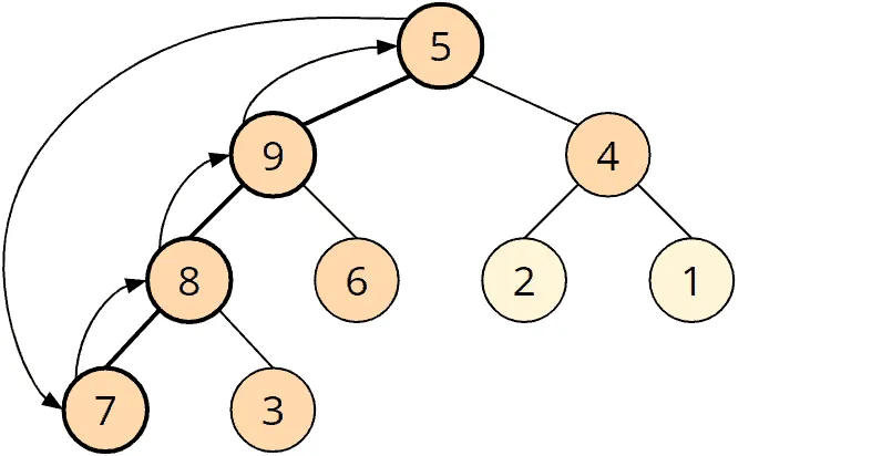
In the end, this leads to the same result as the regular heapify().

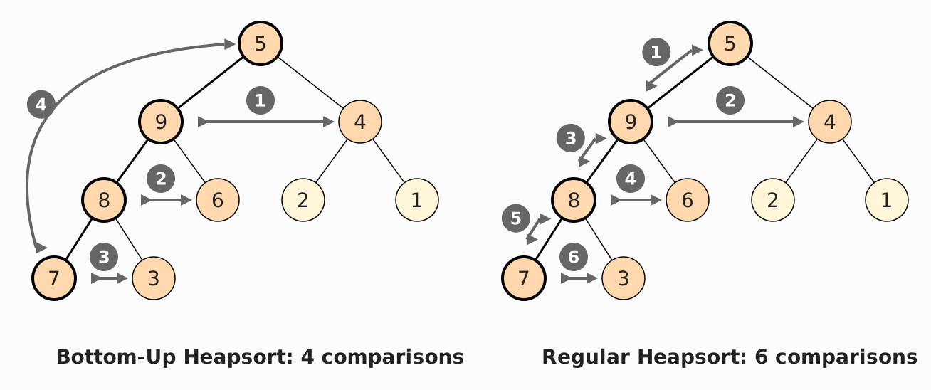
Bottom-Up Heapsort takes advantage of the fact that the root element is usually shifted very far down. The reason is that it comes from the end of the tree after each iteration and is therefore usually small.

This means that fewer comparisons are necessary if one comparison per node is made all the way down and then a short distance up again – compared to two comparisons per node from top to bottom. The following picture shows both variants using the example above; the numbers on the arrows give the order of the comparisons:

Bottom-Up Heapsort Source Code

The class BottomUpHeapsort inherits from Heapsort and overrides its heapify() method with the following:

@Override
void heapify(int[] heap, int length, int rootPos) {
  int leafPos = findLeaf(heap, length, rootPos);
  int nodePos = findTargetNodeBottomUp(heap, rootPos, leafPos);

  if (rootPos == nodePos) {
    return;
  }

  // Move all elements starting at nodePos to parent, move root to nodePos
  int nodeValue = heap[nodePos];
  heap[nodePos] = heap[rootPos];

  while (nodePos > rootPos) {
    int parentPos = getParentPos(nodePos);
    int parentValue = heap[parentPos];
    heap[parentPos] = nodeValue;
    nodePos = parentPos;
    nodeValue = parentValue;
  }
}

The findLeaf() method compares two children and follows the larger one until the end of the tree is reached (or a node with only one child):

int findLeaf(int[] heap, int length, int rootPos) {
  int pos = rootPos;
  int leftChildPos = pos * 2 + 1;
  int rightChildPos = pos * 2 + 2;

  // Do two children exist?
  while (rightChildPos < length) {
    if (heap[rightChildPos] > heap[leftChildPos]) {
      pos = rightChildPos;
    } else {
      pos = leftChildPos;
    }
    leftChildPos = pos * 2 + 1;
    rightChildPos = pos * 2 + 2;
  }

  // Does one child exist?
  if (leftChildPos < length) {
    pos = leftChildPos;
  }

  return pos;
}

The method findTargetNodeBottomUp() searches from bottom to top for the first element that is not smaller than the root node:

int findTargetNodeBottomUp(int[] heap, int rootPos, int leafPos) {
  int parent = heap[rootPos];
  while (leafPos != rootPos && heap[leafPos] < parent) {
    leafPos = getParentPos(leafPos);
  }
  return leafPos;
}

And finally the getParentPos() method:

int getParentPos(int pos) {
  return (pos - 1) / 2;
}

Bottom-Up Heapsort Performance

We can also measure the performance of Bottom-Up Heapsort with UltimateTest; the numbers come from the same run as the table above:

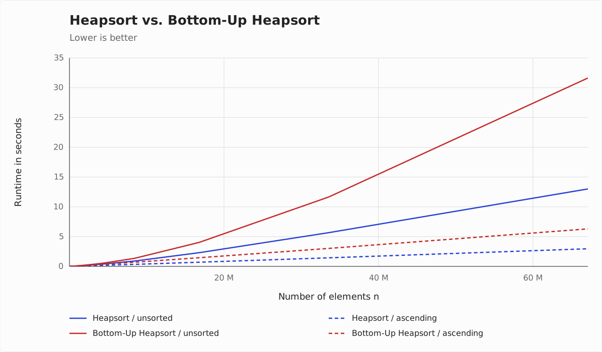
So Bottom-Up Heapsort is slower than regular Heapsort – and the larger the array, the clearer the difference:

• For unsorted data, both are equally fast up to 65,536 elements (a difference of at most 3%). After that, Bottom-Up Heapsort falls behind and takes 2.4 times as long at 67,108,864 elements.
• For sorted data, Bottom-Up Heapsort takes about twice as long at 67,108,864 elements (2.1 times for ascending, 2.0 times for descending order).

In 2020, things looked different: Back then, Bottom-Up Heapsort was faster for unsorted data up to about one million elements and at most 6% slower for sorted data.

Why Is Bottom-Up Heapsort Slower?

It is not the number of operations: According to CountOperations, Bottom-Up Heapsort needs fewer compare, read, and write operations than regular Heapsort. It does go through the tree twice – down and a short way back up – and therefore needs 1.8 to 1.9 times as many loop iterations. But this ratio is almost the same for every array size and does not explain the growing gap.

Nor does the way back up cost memory accesses: At 67,108,864 elements, the way down is 26 levels deep, and since the two children of a level lie in at most two cache lines, it reads at most 52 cache lines of 128 bytes each, just under 7 KB. These are still in the L1 cache on the way back up, which on the M5 Pro is 64 or 128 KB in size, depending on the core.

The difference lies in how the two variants descend the tree. At each level, both need to know which child is larger before they can continue:

• Heapsort guesses. The comparison is a conditional branch, and the processor predicts its outcome – the branch prediction from above. This way, it can already load the next level before the comparison is finished. If it guesses wrong, it has to start over; if it guesses right, it has gained time.
• Bottom-Up Heapsort waits. The JIT compiler translates the choice of the larger child in findLeaf() without a branch (on ARM, with the csel instruction). There is nothing to guess – but the next level can only be loaded once both children have been loaded and compared. Each step waits for the previous one.

The processor’s performance counters, which I read while sorting, show the effect (details in the info box below). The values are per element, at 67,108,864 elements:

Variant, input	Cycles	L1 cache misses	Cycles waiting for misses	Branch mispredictions
Heapsort, unsorted	873	26.3	226	13.5
Bottom-Up, unsorted	2,098	23.6	1,528	0.8
Heapsort, ascending	196	0.3	1.0	3.6
Bottom-Up, ascending	404	0.1	0.8	0.1

With these numbers, each of the three cases in the diagram can be explained:

• Large unsorted arrays: Both variants miss the L1 cache about equally often. Heapsort guesses wrong at about every second level, but with every right guess it loads ahead, so that several misses run at the same time. With Bottom-Up Heapsort, they run one after the other: It waits 1,528 cycles per element, Heapsort only 226. This difference makes up the entire gap.
• Sorted data: Here, neither variant waits for memory. Heapsort almost always guesses right and runs at full speed. Bottom-Up Heapsort still has to wait step by step and needs twice as many cycles.
• Small unsorted arrays: Up to 65,536 elements, both hardly miss the L1 cache (at most 1.5 times per element). Heapsort loses time through its wrong guesses, Bottom-Up Heapsort through waiting – both cost about the same, and the variants are equally fast.

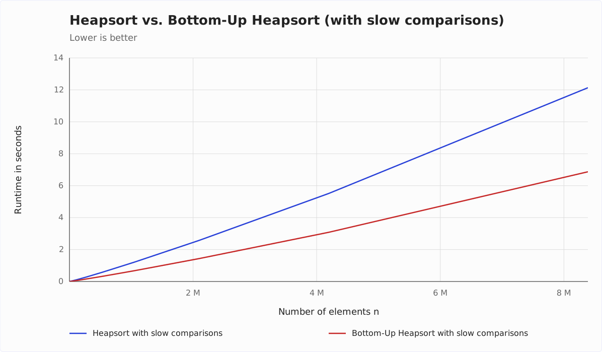
Bottom-Up Heapsort With Expensive Comparison Operations

Bottom-Up Heapsort is optimized to reduce the number of comparisons required. With int primitives, comparisons are not significant, so Bottom-Up Heapsort cannot show its advantages here.

I have, therefore, carried out another test by artificially increasing the cost of the comparison operations. You can find the adapted algorithms in the classes HeapsortSlowComparisons and BottomUpHeapsortSlowComparisons in the GitHub repository.

They slow down each comparison with Thread.onSpinWait(). On x86 processors, the JIT compiler translates this call into the PAUSE instruction, which makes the processor wait briefly. On the Apple M5, JDK 27 generates a YIELD instruction instead, which costs practically nothing there – without further measures, the slow variants are as fast as the ones without the slowdown. For the measurement, I therefore had the JVM generate four ISB instructions (instruction barriers) per call; the JVM options are in the info box below.

Bottom-Up Heapsort performs significantly better in this comparison – from 16,384 elements on, it is 1.74 to 1.79 times as fast as regular Heapsort:

Further Characteristics of Heapsort

In the following sections, we look at the space complexity of Heapsort, its stability, and parallelizability.

Space Complexity of Heapsort

Heapsort is an in-place sorting method, i.e., no additional memory space is required except for loop and auxiliary variables. The number of these variables is always the same, whether we sort ten elements or ten million. Therefore:

The space complexity of Heapsort is: O(1).

Stability of Heapsort

It is easy to construct examples that show that elements with the same key can change their position to each other:

Example 1

When we sort the array [3, 2a, 2b, 1] with Heapsort, we perform the following steps (2a and 2b represent two elements with the same key; highlighted in light yellow are the elements that will be swapped in the next step; highlighted in blue are finished elements):

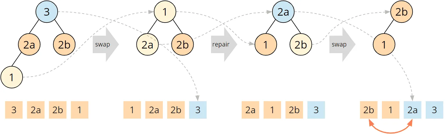
At this point, we can abort because we can already see that the target array will end in [2a, 3], i.e., 2a will end up to the right of 2b in the target array.

Adjust the algorithm?

In the second step, we swapped the 1 with the 2a according to the algorithm. Could we change the algorithm so that for child nodes with the same key, the parent is not swapped with the left child, but with the right one?

In that case, the array above would be sorted stably because the 1 would not be swapped with the 2a, but with the 2b. And then, the 2b would end up at the second-to-last position of the array.

Example 2

Let’s try this with another input array, with [4, 3, 2a, 2b, 1]:

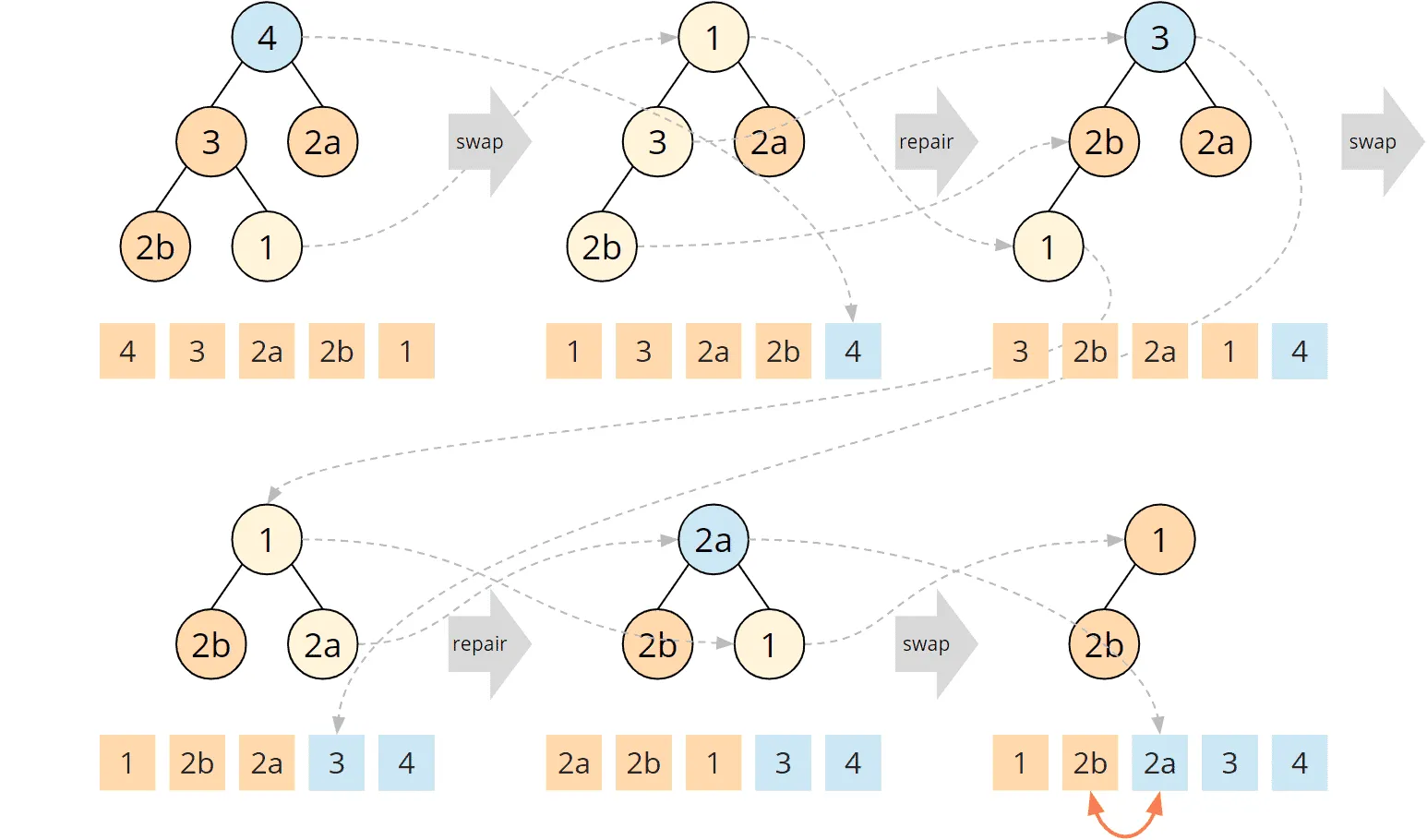
After step 2, we have reached the state we had before as the initial array, with 2a and 2b having swapped their positions. If we now exchange 1 with the right child in the next step, the same thing happens as above: 2a arrives first in the target array and thus ends up to the right of 2b.

We have shown counterexamples for both algorithm variants and can therefore state:

Heapsort is not a stable sorting algorithm.

Heapsort Parallelizability

With Heapsort, the whole array is continuously changing, so there are no apparent solutions to parallelize the algorithm.

Comparing Heapsort With Other Efficient Sorting Algorithms

The following diagram shows the runtimes of Heapsort compared to those of Quicksort and Merge Sort, measured on the same machine. The numbers for Quicksort and Merge Sort come from a run on September 27, 2026; Quicksort uses the middle element as the pivot, as in the 2020 measurement:

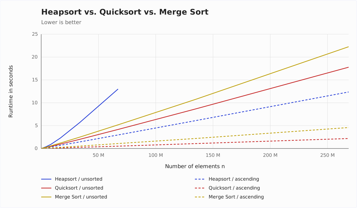
For 67,108,864 randomly distributed elements, Heapsort takes 13.0 seconds, Quicksort 4.2, and Merge Sort 5.2 seconds. Heapsort thus takes 3.1 times as long as Quicksort and 2.5 times as long as Merge Sort (in 2020: 3.6 and 2.4 times). For data sorted in ascending order, Heapsort takes 5.7 to 6.2 times as long as Quicksort from 16,384 elements on (in 2020: eight to nine times) and 2.7 to 2.9 times as long as Merge Sort (in 2020: two times).

Heapsort vs. Quicksort

As shown in the previous section, Quicksort is usually much faster than Heapsort.

Due to the O(n²) worst-case time complexity of Quicksort, Heapsort is sometimes preferred to Quicksort in practice.

As shown in the article about Quicksort, if the pivot element is chosen appropriately, the worst case is unlikely to occur. Nevertheless, there is a certain risk that a potential attacker with sufficient knowledge of the Quicksort implementation used can exploit this knowledge to crash or freeze an application with appropriately prepared input data.

That is why the Java class library combines both algorithms: Since Java 14, Arrays.sort() switches from Dual-Pivot Quicksort to Heapsort for int, long, float, and double arrays as soon as the recursion gets too deep. This keeps the runtime at O(n log n) even for prepared input data. This principle – Quicksort with Heapsort as an “emergency brake” – is called Introsort.

There is no JEP for this change; it is tracked in the bug tracker under JDK-8226297.

Heapsort vs. Merge Sort

Merge Sort is also usually faster than Heapsort. Besides, unlike Heapsort, Merge Sort is stable.

Heapsort has an advantage over Merge Sort in that it does not require additional memory, while Merge Sort requires additional memory in the order of O(n).

Summary

Heapsort is an efficient, unstable sorting algorithm with an average and worst-case time complexity of O(n log n). Only when all elements are equal does heapify() stop right away – then Heapsort sorts in O(n).

Heapsort is significantly slower than Quicksort and Merge Sort. You will therefore rarely find it as a standalone sorting algorithm, but you will find it as an “emergency brake”: Since Java 14, Arrays.sort() switches to it when Quicksort recurses too deeply on an int, long, float, or double array.

By the way: the Java class PriorityQueue uses the same kind of binary heap that Heapsort builds in phase 1 as its internal data structure.

You will find more sorting algorithms in the overview of all sorting algorithms and their characteristics in the first part of the article series.