Shortest Path Algorithms in Java: Overview + Maze Example

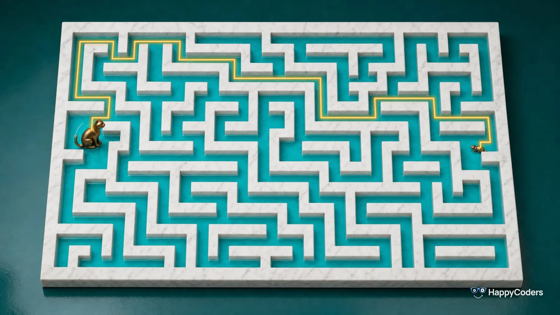
How does a sat-nav system find the shortest path from start to destination? How do bot opponents orient themselves in first-person shooters? This series of articles on shortest path algorithms (and more generally: pathfinding algorithms) will address these questions.

This first article covers the following topics:

• What is the difference between “Shortest Path” and “Pathfinding”?
• Which shortest path algorithms exist?
• How to find the shortest path between two points in a maze?

You can find the source code for the article in my GitHub repository.

Shortest Path or Pathfinding?

A shortest path algorithm solves the problem of finding the shortest path between two points in a graph (e.g., on a road map). The term “short” does not necessarily mean physical distance. It can also be time (freeways are preferred) or cost (toll roads are avoided), or a combination of multiple factors.

Graphs can be very complex and contain millions of nodes and edges (for example, in a video game world where hundreds or thousands of characters can move around freely), so finding the optimal path would be very time-consuming.

For certain applications, it is sufficient to find a reasonably short (or even any) way. That is then generally referred to as pathfinding.

Shortest Path Algorithms

The best known shortest path algorithms are:

• Dijkstra’s algorithm
• the A* search algorithm (pronounced “A Star”)
• the Bellman-Ford algorithm
• the Floyd-Warshall algorithm

On two-dimensional, tile-based maps, such as those used in early computer games, we can also use a form of breadth-first search known as the Lee algorithm.

In the remaining part of this article, I explain an optimized version of the Lee algorithm using an example with animations and Java source code.

Maze Algorithm: How to Find the Shortest Path in a Labyrinth?

My favorite example for solving the shortest path problem is the game “FatCat” on the HP-85, a computer from the 1980s. My uncle let me experiment with this computer as a child.

The mission was (like in Pac-Man) to let a mouse eat all the cheese pieces in a maze – without being eaten by the cat. The difficult part was (apart from the control with only two buttons to turn the mouse left and right) that the cat (unlike the ghosts in Pac-Man) always took the shortest path to the mouse.

Only through a mouse hole connecting the left and right edges could one evade the cat. Besides, the mouse could be beamed to a different location once per life – which was especially helpful in dead ends:

At that time (I was about ten years old), I was already interested in programming and wanted to reprogram the game on my C64. I had quickly implemented the display of the mazes and the control of the mouse. But calculating the shortest path between cat and mouse caused me headaches for months.

In the end, I solved it – as I was to find out years later in my computer science studies – with a variant of the Lee algorithm. Without knowledge of this algorithm, I had developed an optimized variant of it, which I will present step by step in the following chapters.

Optimized Lee Algorithm

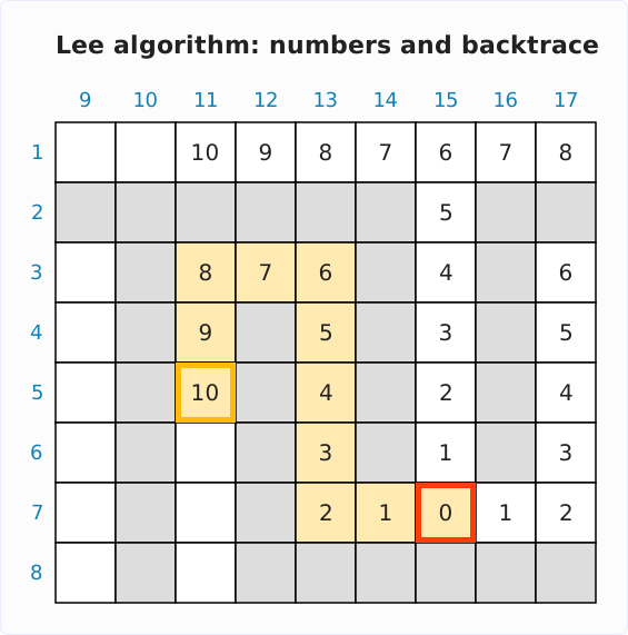
The Lee algorithm works in two phases. First, it numbers the fields round by round, beginning at the start: the start gets the number 0, all free neighboring fields get 1, their unmarked neighbors get 2 – until the target has a number.

Then it walks back from the target, each time to the neighboring field whose number is one lower, until it reaches the start again – because the numbers only tell how far a field is from the start, not which direction the cat has to take from the start. This way back is called the backtrace.

The following diagram shows both phases on a section of the labyrinth shown above. The numbering starts at the cat (framed in red) and ends as soon as the mouse (framed in yellow) gets the number 10. The backtrace from the mouse back to the cat is highlighted in yellow.

If the numbering starts at the cat, the cat’s first step is known only when the backtrace arrives back at the cat.

There are two ways to avoid this: either the numbering starts at the mouse – then the cat’s neighboring field whose number is one lower shows the direction. Or you start at the cat and remember for every field the direction in which the cat set off from its starting position.

The following diagram shows both ways on the same section. On the left, the numbering starts at the mouse. The cat gets the number 10, and its only neighboring field with the number 9 is highlighted in yellow – to its left. On the right, every field discovered by the time the mouse is found shows the cat’s initial direction. The field above the mouse is highlighted in yellow: its direction, left, is the answer.

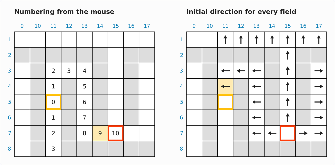
The variant in this article takes the second way. The four directions fit into two bits; the number of a field needs more. Today, that makes no difference, but in 1990, I still paid attention to every bit.

There is one thing the Lee algorithm does not specify: how to find the “neighbors of points marked with i”. It would be quite slow to search the whole labyrinth at every step. At this point, I use a queue known from the breadth-first search to store the fields to process in the next step.

All images and animations in this section use the labyrinth shown above with the cat at position (15,7) and the mouse at position (11,5). The coordinate system starts at the upper left corner of the labyrinth with (0,0).

Preparation

The maze is stored in a two-dimensional boolean array called lab. Walls are identified by the value true. Keeping the outer wall in this array simplifies the code, which does not need separate checks for reaching the edges.

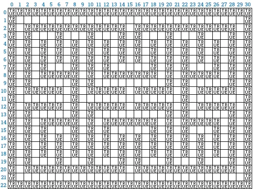
To avoid running in circles, we create another two-dimensional boolean array named discovered, in which we mark the fields we have already discovered during the search. The current position of the cat is initially set to true.

The labyrinth walls are colored gray, the position of the cat is marked red, and that of the mouse yellow. The discovered array does not contain this information. It is shown below for easier understanding.

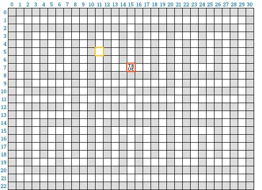
Furthermore, we create the queue for the fields to be visited next. We insert the current position of the cat (15,7) into the queue without a direction (therefore null):

You can learn all about queues in the HappyCoders Queue Tutorial.

Step 1

We remove the element just put into the queue (the start position of the cat):

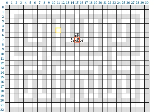
Then we write all fields the cat can reach in one step into the queue – with their X and Y coordinates and the respective direction relative to the starting point:

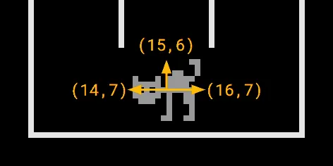
These fields are also marked as “discovered”:

Steps 2 to n

As long as the queue is not empty, we now take one position element at a time and write all fields reachable from this position into the queue – unless they are already marked as “discovered”.

This time, we don’t save the direction taken in this step. Instead, we copy the direction from the removed element. After all, we want to know which direction the cat must take from its starting position.

The first element in the queue is the position (15,6) above the cat:

From this position, we can reach the fields above (15,5) and below (15,7):

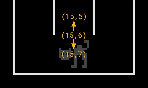
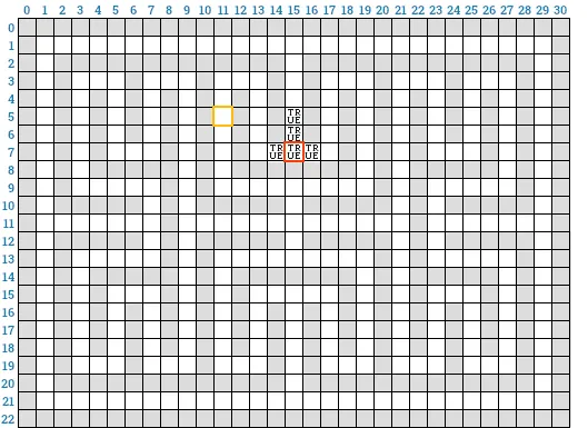
The lower field (15,7) is already marked as “discovered” (that is where we came from), and it will be ignored. We write the upper field (15,5) into the queue and also mark it as “discovered”:

We will now repeat this process until we reach the position of the mouse. The following animation shows how the discovered array fills up step by step:

Termination Condition

As soon as we reach the position of the mouse, the algorithm is finished. The queue entry removed last indicates the direction in which the cat has to go. In the example, that is (11,4)/LEFT (the field above the mouse):

Thus the shortest path from cat to mouse leads to the left. In the following image, I have highlighted the path in yellow:

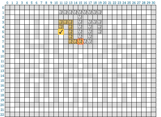
The path can no longer be inferred from the data at this point. It is irrelevant because the cat has to take only one step, and after that, the shortest path is calculated again (because the mouse is moving too, and the shortest path could lead in a different direction in the next step).

If the queue is empty without the mouse being found, there is no path between cat and mouse. This case cannot occur in the FatCat game but should be handled for other applications.

Since every field is marked as “discovered” before it enters the queue, each free field enters the queue at most once. For every field taken from the queue, the algorithm checks four neighbors. The running time therefore grows linearly with the size of the labyrinth: O(w · h) for a width w and a height h – in the example, at most 31 · 23 = 713 fields.

Shortest Path Java Code

The following code implements the algorithm with modern language features and data structures like the ArrayDeque as a queue. You can find it in the GitHub repository in the CatAlgorithmFrom2020 class.

You will find the code of the Direction enum at the end.

/**
 * Finds the shortest path from cat to mouse in the given labyrinth.
 *
 * @param lab the labyrinth's matrix with walls indicated by {@code true}
 * @param cx the cat's X coordinate
 * @param cy the cat's Y coordinate
 * @param mx the mouse's X coordinate
 * @param my the mouse's Y coordinate
 * @return the direction of the shortest path
 */
private Direction findShortestPathToMouse(
    boolean[][] lab, int cx, int cy, int mx, int my) {
  // Create a queue for all nodes we will process in breadth-first order.
  // Each node is a data structure containing the cat's position and the
  // initial direction it took to reach this point.
  Queue<Node> queue = new ArrayDeque<>();

  // Matrix for "discovered" fields
  // (I know we're wasting a few bytes here as the cat and mouse can never
  // reach the outer border, but it will make the code easier to read. Another
  // solution would be to not store the outer border at all - neither here nor
  // in the labyrinth. But then we'd need additional checks in the code
  // whether the outer border is reached.)
  boolean[][] discovered = new boolean[lab.length][lab[0].length];

  // "Discover" and enqueue the cat's start position
  discovered[cy][cx] = true;
  queue.add(new Node(cx, cy, null));

  while (!queue.isEmpty()) {
    Node node = queue.poll();

    // Go breadth-first into each direction
    for (Direction dir : Direction.values()) {
      int newX = node.x() + dir.getDx();
      int newY = node.y() + dir.getDy();
      Direction newDir = node.initialDir() == null ? dir : node.initialDir();

      // Mouse found?
      if (newX == mx && newY == my) {
        return newDir;
      }

      // Is there a path in the direction (= is it a free field in the labyrinth)?
      // And has that field not yet been discovered?
      if (!lab[newY][newX] && !discovered[newY][newX]) {
        // "Discover" and enqueue that field
        discovered[newY][newX] = true;
        queue.add(new Node(newX, newY, newDir));
      }
    }
  }

  throw new IllegalStateException("No path found");
}

private record Node(int x, int y, Direction initialDir) {}

And the Direction enum:

public enum Direction {
  UP(0, -1),
  RIGHT(1, 0),
  DOWN(0, 1),
  LEFT(-1, 0);

  private final int dx;
  private final int dy;

  Direction(int dx, int dy) {
    this.dx = dx;
    this.dy = dy;
  }

  public int getDx() {
    return dx;
  }

  public int getDy() {
    return dy;
  }
}

You can test the code with the CatAlgorithmsDemo class. This class creates a maze, places cat and mouse at random positions, and lets the cat move to the mouse on the shortest path.

The demo program visualizes the maze with ASCII blocks. The individual steps are printed one below the other for simplicity (the pathfinding algorithm is in focus here, not the visualization). The following animation shows the printed steps in animated form:

Algorithm Performance

The CatAlgorithmsBenchmark tool allows you to compare the performance of the old and new implementation. The following table shows the median of the measurements from 20 test iterations, each with 100,000 calculations of the shortest path. Ten warmup iterations preceded the test.

Algorithm	Time for 100,000 path calculations
CatAlgorithmFrom1990	163 ms
CatAlgorithmFrom2020	257 ms

At first glance, the algorithm I wrote as a 15-year-old is faster than my new algorithm. How is this possible?

Optimization for FatCat Mazes

Another look into the old code shows that the pathfinding algorithm examines only every second waypoint. This makes sense because the structure of the labyrinths allows the cat to change its direction only after every second step:

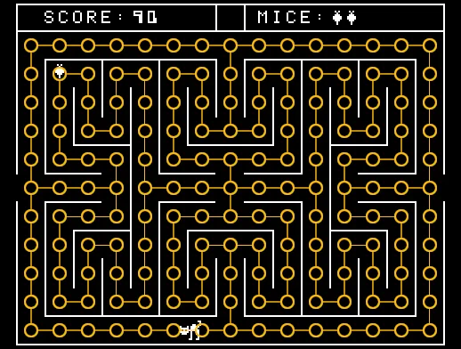
I have optimized the Java code once more. Only the part inside the loop changes. The cat’s intermediate steps must not be ignored completely, though – the mouse could sit there.

You will find the optimized code in the following listing and the CatAlgorithmFrom2020Opt class in the GitHub repository.

while (!queue.isEmpty()) {
  Node node = queue.poll();

  // Go *two* steps breadth-first into each direction
  for (Direction dir : Direction.values()) {
    // First step
    int newX = node.x() + dir.getDx();
    int newY = node.y() + dir.getDy();
    Direction newDir = node.initialDir() == null ? dir : node.initialDir();

    // Mouse found after first step?
    if (newX == mx && newY == my) {
      return newDir;
    }

    // Is there a path in the direction (= is it a free field in the labyrinth)?
    // No -> continue to next direction
    if (lab[newY][newX]) continue;

    // Second step
    newX += dir.getDx();
    newY += dir.getDy();

    // Mouse found after second step?
    if (newX == mx && newY == my) {
      return newDir;
    }

    // Target field has not yet been discovered?
    if (!discovered[newY][newX]) {
      // "Discover" and enqueue that field
      discovered[newY][newX] = true;
      queue.add(new Node(newX, newY, newDir));
    }
  }
}

And here is the result of another performance comparison:

Algorithm	Time for 100,000 path calculations
CatAlgorithmFrom1990	163 ms
CatAlgorithmFrom2020	257 ms
CatAlgorithmFrom2020Opt	138 ms

The new code is now about 15% faster than the code from 1990.

If you have looked into the code from 1990: The reason for the difference is that I did not use a queue back then, but two separate data structures for the starting and ending points of each pathfinding step. After each step, all discovered ending points were copied back into the starting points’ data structure.

May I be forgiven for not thinking about using a queue (which I couldn’t have simply pulled out of the toolbox at that time anyway) when I was 15 ;-)

Summary and Outlook

This article described the “shortest path problem” and used the “FatCat” game (by the way, we called it “cat and mouse”) as an example to show how to solve the problem with a pathfinding algorithm in Java.

The algorithm presented here can only be applied to tile-based maps or to graphs that represent tile-based maps.

The following parts of the series introduce the general shortest path algorithms: Dijkstra’s algorithm, the A* search algorithm, the Bellman-Ford algorithm, and the Floyd-Warshall algorithm.