Floyd-Warshall Algorithm: Matrix Example, Java Code, Complexity

In this series about pathfinding algorithms, you have read about Dijkstra’s algorithm, the A* algorithm, and the Bellman-Ford algorithm. This last part will show you how the Floyd-Warshall algorithm (also known as Floyd’s algorithm) works and what it is used for.

I will address the following topics in detail:

• What is the intended use of the Floyd-Warshall algorithm?
• How does the Floyd-Warshall algorithm differ from the pathfinding algorithms presented so far?
• How does the Floyd-Warshall algorithm work (explained step by step with an example)?
• How to implement the Floyd-Warshall algorithm in Java?
• How to determine the time complexity of the Floyd-Warshall algorithm?

You can find the source code for the entire article series on pathfinding algorithms in this GitHub repository.

When to Use the Floyd-Warshall Algorithm?

All pathfinding algorithms presented so far find the shortest path from a single source node to a destination node (or to all other nodes of a graph).

Dijkstra prioritizes the search by total cost from the starting node. A* prioritizes additionally according to estimated remaining costs to the target. And Bellman-Ford does not prioritize at all but can handle negative edge weights.

Floyd-Warshall, on the other hand, finds the shortest paths between all pairs of start and destination nodes (Floyd’s variant).

Like Bellman-Ford, Floyd-Warshall can handle negative edge weights – as long as the graph contains no negative cycle. How the algorithm detects such a cycle is explained in the section Detecting Negative Cycles in the Graph.

For an undirected graph, you enter each edge in both directions. A negative undirected edge, however, is then already a negative cycle: it leads from one node to the other and back again at negative cost.

Transitive Closure of a Graph

Alternatively, Floyd-Warshall computes the so-called “transitive closure” of a graph (Warshall’s variant). The transitive closure extends a graph by edges between all indirectly connected pairs of nodes. For example, if the graph has two edges – one from A to B and one from B to C – then the transitive closure extends the graph by the edge from A to C (since a path from A to C via B exists).

The following graphic shows a somewhat more complex example with four nodes – the initial graph on the left and its transitive closure on the right. The blue arrows represent the added, indirect connections:

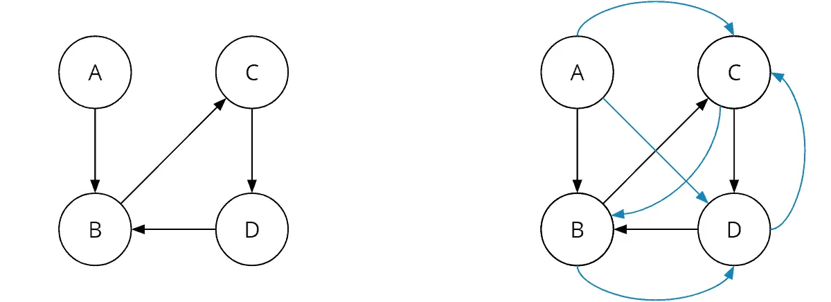
Both tasks are very similar: If a shortest path exists between two nodes, then this node pair also belongs in the transitive closure – and vice versa. Therefore, the variants of Floyd and Warshall are combined into a single algorithm.

Robert Floyd and Stephen Warshall both published their variants in 1962. Bernard Roy had already described the same algorithm in 1959.

How Does the Floyd-Warshall Algorithm Work?

The algorithm is easy to implement, as you will see later. However, the explanation is a bit tricky. I will, therefore, first describe the algorithm with an example.

Floyd-Warshall Algorithm – Example

The following example graph contains five nodes, labeled A, B, C, D, E, and various directed and weighted edges:

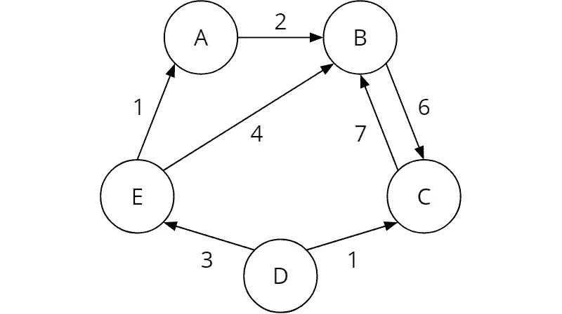
The numbers on the edges (the edge weights) represent the costs for the respective path. For example, the cost from E to B is 4.

Preparation – Node Pair Matrix

In preparation, we create an n × n matrix (n is the number of nodes) in which we enter – for each pair of nodes (i, j) – the weight of the edge from i to j if it exists. Otherwise, we enter infinity (∞). On the diagonal (the distance of a node to itself), we enter 0.

from / to	A	B	C	D	E
A	0	2	∞	∞	∞
B	∞	0	6	∞	∞
C	∞	7	0	∞	∞
D	∞	∞	1	0	3
E	1	4	∞	∞	0

From the table, we can read, for instance: The cost from A to B is 2 (row A, column B).

Floyd-Warshall Algorithm – Step by Step

We now perform the following five iterations. In each case, we examine one of the nodes as a potential intermediate node.

Iteration 1 – Indirect Paths via Intermediate Node A

For all node pairs (i, j), we compare the entered costs of the direct path with the costs of the indirect path from i to j via node A – i.e., the costs from node i to node A plus the costs from node A to node j (if such a path exists). If the costs via intermediate node A are lower than the previous ones, we replace the costs in the matrix.

Node pairs where i = j or i = A or j = A can be skipped. The distance of a node to itself is always 0. And if start or destination are already A, there is not also an indirect path via A.

We thus start with the node pair (B, C). The cost of the direct path is 6 (row B, column C). There is currently no known path from B to A (row B, column A contains infinity). So we cannot find a shorter route via A in this iteration. Accordingly, we cannot find shorter paths for (B, D) and (B, E) via A.

Also, from C and D, there are currently no known paths to node A (column A contains infinity for both rows C and D). Thus, we cannot currently find shorter routes for (C, B), (C, D), (C, E), (D, B), (D, C), (D, E).

At the node pair (E, B), things start to get interesting. The current cost of the direct path E→B is 4. Is there a shorter route via node A? Here is the corresponding section of the graph:

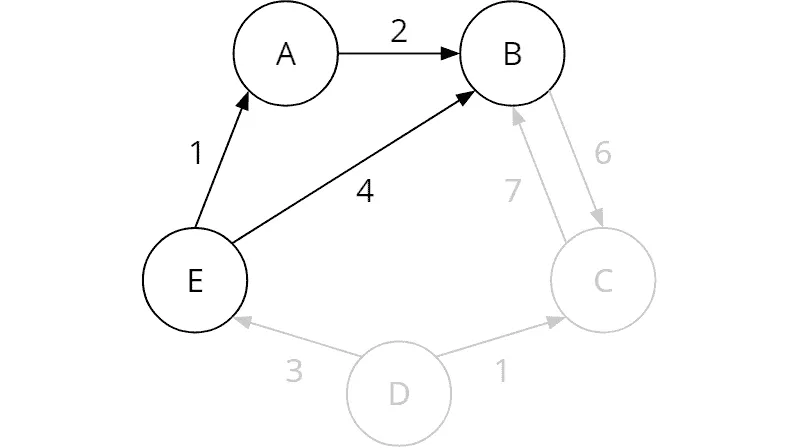
The cost from E to A is 1 (row E, column A in the table); the cost from A to B is 2 (row A, column B). These add up to 3. The cost of the indirect path from E to B via node A is, therefore, lower than that of the direct path. So we have found the following, shorter path:

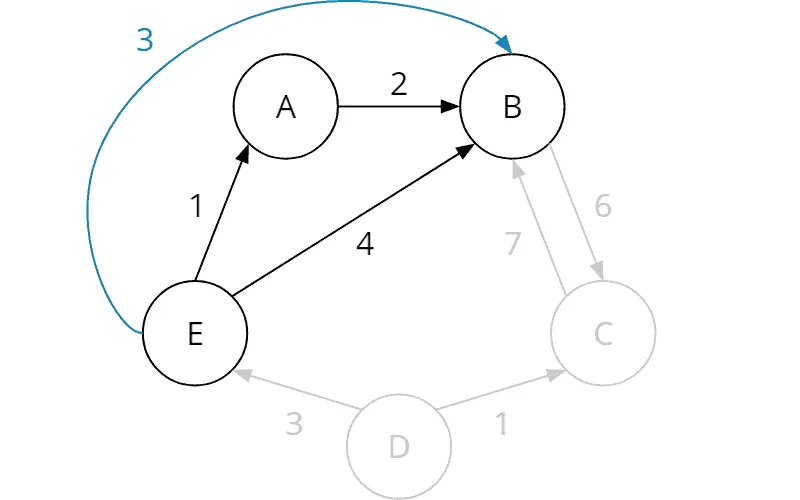
We, therefore, replace the 4 in row E, column B with a 3 (highlighted in bold in the table):

from / to	A	B	C	D	E
A	0	2	∞	∞	∞
B	∞	0	6	∞	∞
C	∞	7	0	∞	∞
D	∞	∞	1	0	3
E	1	3	∞	∞	0

Next, we examine node pair (E, C). The current cost is infinity since no path has been found yet. Is there an indirect path via A, i.e., E→A→C? Since no path from A to C is currently known (row A, column C contains infinity), the answer is “no”.

Finally, we look at the node pair (E, D). Since no path is known from A to D, we cannot find an indirect way E→A→D in this iteration.

We have examined all node pairs; iteration 1 is now complete. We now know the lowest cost for all node pairs if we also allow indirect paths via intermediate node A. In particular, we have found a shorter route from E to B via node A in this iteration.

Iteration 2 – Indirect Paths via Intermediate Node B

In the second iteration, we compare the costs entered for all node pairs (i, j) (these are now either the costs of the direct path or those via intermediate node A – whichever is lower) with the costs from i to j via node B.

We read the costs to and from node B from the matrix. This means that these do not necessarily have to be the costs of the direct path to/from node B. It could also be the lower costs via intermediate node A determined in iteration 1 (e.g., from E to B: 3 via A instead of 4 directly).

We start with node pair (A, C). So far, no path has been found (row A, column C contains infinity). Let’s look at the indirect route via B:

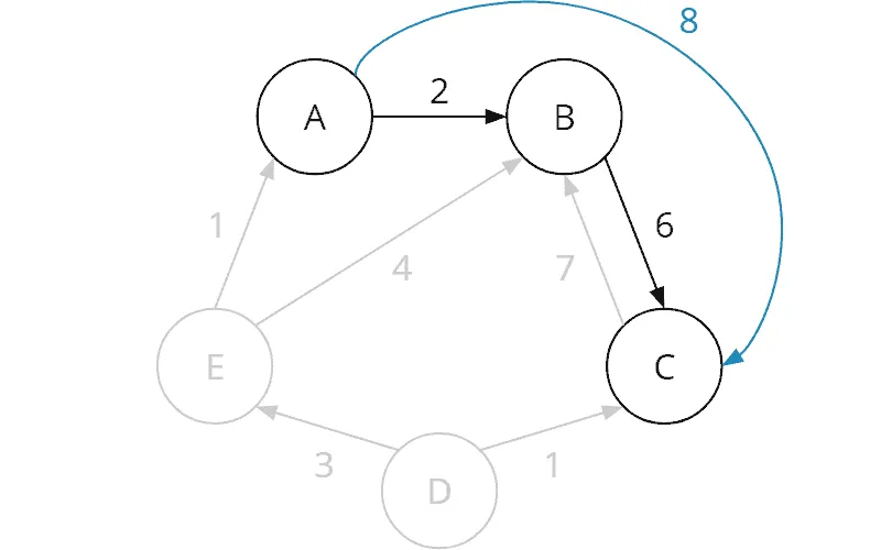
The cost from A to B is 2, and the cost from B to C is 6. The sum is 8. This is better than no path at all. We, therefore, enter the 8 in row A, column C:

from / to	A	B	C	D	E
A	0	2	8	∞	∞
B	∞	0	6	∞	∞
C	∞	7	0	∞	∞
D	∞	∞	1	0	3
E	1	3	∞	∞	0

We continue with node pair (A, D). Here, too, no path is known so far. Is there a route via intermediate node B? We have just read the costs from A to B as 2. From B to D, however, no path is known so far. Thus, we cannot determine any costs for route A→B→D, and the entry for node pair (A, D) remains unchanged (infinity).

The same happens with node pair (A, E): there is a path A→B, but no path B→E, hence no path A→B→E and therefore no new entry for node pair (A, E).

We come to the node pairs (C, A), (C, D), and (C, E): Currently, no path is known for any of the three pairs. There is a path C→B with a cost of 7, but there is no path from intermediate node B to A, D, or E, so there can be no paths C→B→A, C→B→D, or C→B→E. Therefore, the entries for the three node pairs remain unchanged (infinity).

Node pairs (D, A), (D, C), and (D, E): Since there is no path from node D to intermediate node B, we cannot find any (or any shorter) paths for these three node pairs either.

Node pair (E, A): There is a path from E to B, but none from B to A, hence no path E→B→A.

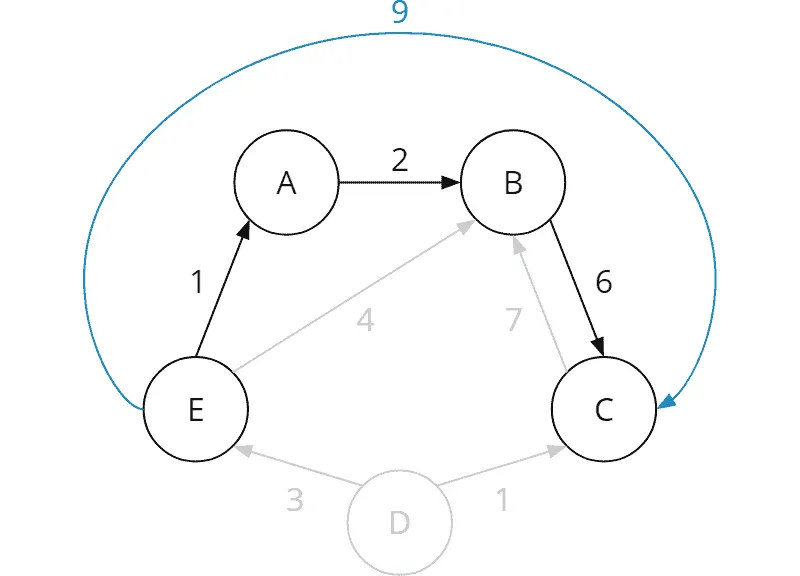
Node pair (E, C) provides some momentum again: Currently, no path is known. Is there a route via B? There is a path E→B with a cost of 3 and a path B→C with a cost of 6. Thus, there is a path from E via B to C with a total cost of 9. We enter the 9 in row E, column C:

from / to	A	B	C	D	E
A	0	2	8	∞	∞
B	∞	0	6	∞	∞
C	∞	7	0	∞	∞
D	∞	∞	1	0	3
E	1	3	9	∞	0

Note that this does not mean that the route from E to C has to go only via node B. After all, the path from E to B with cost 3 also goes via node A (which we had found in iteration 1). Strictly speaking, we have now found the path E→A→B→C:

Let us examine the last node pair in this iteration: (E, D). Does a route exist via intermediate node B? There is a path E→B with cost 3, but no path B→D, so there is no path E→B→D.

The second iteration is finished. We now know the lowest cost for all node pairs if we also allow indirect paths via node B – and indirectly via node A.

Iteration 3 – Indirect Paths via Intermediate Node C

We repeat the whole thing: Now, we compare for all node pairs the entered costs with those via intermediate node C. The costs to/from node C, which we again read from the matrix, can be those of the direct path to/from node C – but also the costs of indirect routes via node A and/or B determined in the previous iterations.

We start with node pair (A, B). The costs from A to intermediate node C are 8 (we had found this path via B at the beginning of the second iteration). The cost from C to B is 7. The way via intermediate node C thus has a total cost of 8 + 7 = 15. This route is significantly longer than the one currently stored with a cost of 2. You can also see this clearly in the graph: The path A→B is, of course, significantly shorter than A→B→C→B. We, therefore, leave the entry for (A, B) at 2.

Node pairs (A, D) and (A, E): We have just read the costs for A→C, but there are no paths C→D or C→E, so there are none from A via C to D or from A via C to E, respectively.

Node pairs (B, A), (B, D), (B, E): the cost from B to C is 6, but from C, there is no path to A, D, or E. Thus, in this iteration, we do not find any of the paths B→C→A, B→C→D, and B→C→E.

Node pair (D, A): There is a path from D to C, but none from C to A, thus none from D via C to A.

The cost of the node pair (D, B) is currently infinity, i.e., no path is known. That will change now. There is a path D→C with a cost of 1 and a path C→B with a cost of 7, which adds up to 8:

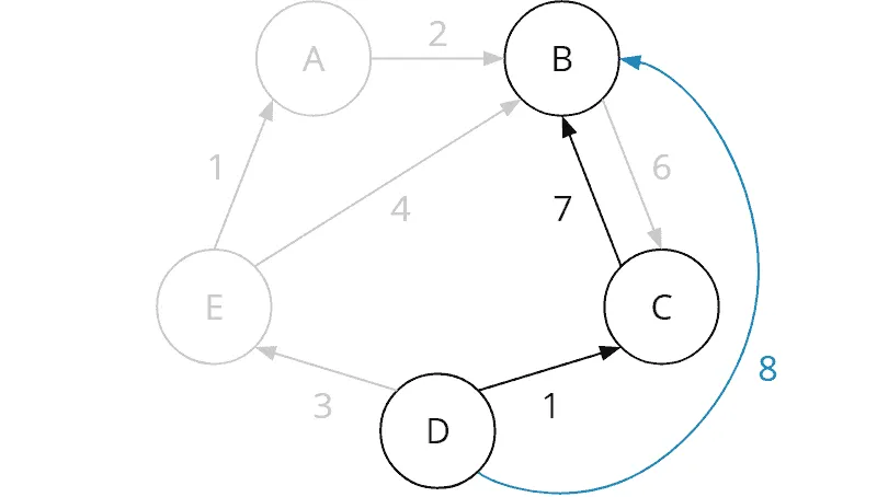
We thus enter 8 in row D, column B:

from / to	A	B	C	D	E
A	0	2	8	∞	∞
B	∞	0	6	∞	∞
C	∞	7	0	∞	∞
D	∞	8	1	0	3
E	1	3	9	∞	0

Node pair (D, E): There is no known path from intermediate node C to E; thus, we do not find a way from D via C to E in this iteration.

Node pairs (E, A) and (E, D): Since there are no paths from intermediate node C to A or D, we currently cannot find a path from E via C to A or from E via C to D respectively.

Node pair (E, B): The cost for path E→C is 9, the cost for C→B is 7, which adds up to 16. For path E→B, a cost of 3 is already stored. 16 is worse, so we leave the 3 unchanged.

Arriving at the end of iteration 3, we know the lowest cost for all node pairs if we also allow indirect paths via node C – and thus via A and B as well.

Iteration 4 – Indirect Paths via Intermediate Node D

We can abbreviate iteration 4: There is no path from any node to intermediate node D. Thus, we will not find a route via D for any node pair.

Iteration 5 – Indirect Paths via Intermediate Node E

In the last iteration, we check for all node pairs if we can find a shorter path via intermediate node E.

We can handle the node pairs with start nodes A, B, and C quickly: There is no path from any of these nodes to intermediate node E, so we will not find a route via E for any of these node pairs.

Node pair (D, A): the cost of path D→E is 3, and the cost of E→A is 1. Thus, there exists a path from D via E to A with a total cost of 4:

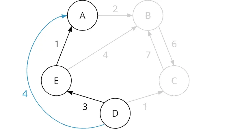
We enter the 4 in row D, column A:

from / to	A	B	C	D	E
A	0	2	8	∞	∞
B	∞	0	6	∞	∞
C	∞	7	0	∞	∞
D	4	8	1	0	3
E	1	3	9	∞	0

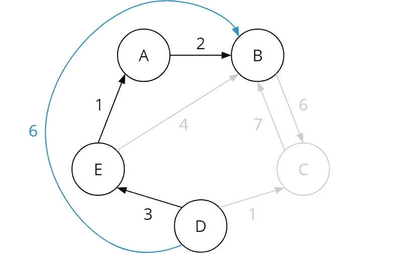
Node pair (D, B): The cost for the path D→E is still 3, the cost for E→B is also 3. That makes a total of 6. We have thus found a path from D via E to B with a total cost of 6. Currently, a total cost of 8 is entered here. We replace the 8 by 6:

from / to	A	B	C	D	E
A	0	2	8	∞	∞
B	∞	0	6	∞	∞
C	∞	7	0	∞	∞
D	4	6	1	0	3
E	1	3	9	∞	0

This case is again an example of the fact that the path via intermediate node E is not the direct path D→E→B, but in fact D→E→A→B, since the shortest path from E to B is via A (we had found the path E→A→B in the first iteration):

The final node pair is (D, C): the cost for path D→E is still 3, the cost for E→C is 9. That makes a total of 12. That is worse than the cost of 1 currently stored for (D, C), which we thus let stand.

We have reached the end of the fifth iteration and now know the lowest cost for all node pairs if we also allow indirect paths via node E (and thus also via A, B, C, D) – that is, via any other nodes.

The goal of the algorithm is thus achieved.

Detecting Negative Cycles in the Graph

What is a negative cycle? And why does it pose a problem? I answered these questions in the article about the Bellman-Ford algorithm. This link leads directly to the corresponding section.

A negative cycle from any node will cause the cost from that node to itself to be negative. The Floyd-Warshall algorithm makes it very easy for us to see this. We can read the cost of all nodes to themselves directly from the matrix diagonal. Here is the matrix from the example above after running through all iterations:

from / to	A	B	C	D	E
A	0	2	8	∞	∞
B	∞	0	6	∞	∞
C	∞	7	0	∞	∞
D	4	6	1	0	3
E	1	3	9	∞	0

The diagonal line (highlighted in bold) contains only zeros. That means that there is no negative cycle.

If there were a negative number in at least one field on the diagonal, a negative cycle would be detected. The algorithm would then terminate with an error message.

Floyd-Warshall Algorithm – Determining the Shortest Paths

In its basic form described above, the Floyd-Warshall algorithm calculates only the cost of the shortest paths between two nodes but not the paths themselves (i.e., over which intermediate nodes the shortest path passes).

However, the algorithm can easily be extended so that it also determines the shortest path between two nodes.

For this, we need a second matrix of size n × n, the so-called “successor matrix”. Here we initially enter, for each node pair (i, j) with an edge from i to j, the end node j. That means that the path from i to j initially goes via the successor j. For all other pairs, we enter “no path” (a dash in the table below).

As soon as we find a shorter path via intermediate node k for any pair (i, j), we copy the current value of the matrix field (i, k) to position (i, j). That means that the path from i to j now leads through the same successor as the path from i to k. The successor can be k itself, but also another intermediate node on the shortest route to k.

In the example above, we would initially populate the successor matrix as follows:

from / to	A	B	C	D	E
A	-	B	-	-	-
B	-	-	C	-	-
C	-	B	-	-	-
D	-	-	C	-	E
E	A	B	-	-	-

In iteration 1, we find a shorter path from E to B via A. The successor of E on the path to A (row E, column A) is A; thus, we also enter A as the successor of E on the path to B (row E, column B):

from / to	A	B	C	D	E
A	-	B	-	-	-
B	-	-	C	-	-
C	-	B	-	-	-
D	-	-	C	-	E
E	A	A	-	-	-

Feel free to try updating the matrix yourself across all five iterations (as an exercise).

To check your result: In iteration 2, you enter a B in field (A, C) and an A in field (E, C). In iteration 3, field (D, B) gets a C, iteration 4 changes nothing, and in iteration 5, fields (D, A) and (D, B) each get an E.

In the end, the successor matrix should look like this (all changes are highlighted in bold):

from / to	A	B	C	D	E
A	-	B	B	-	-
B	-	-	C	-	-
C	-	B	-	-	-
D	E	E	C	-	E
E	A	A	A	-	-

How can we read the shortest paths from this matrix?

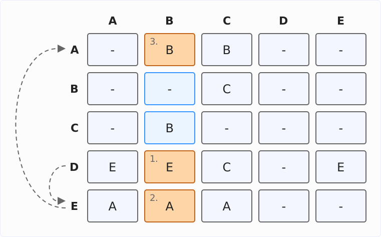
Let’s take the path from D to B that we had calculated in the fifth iteration.

We read from the matrix step by step:

• Row D, column B: The direct successor of D on the route to B is: E
• Row E, column B: The direct successor of E on the route to B is: A
• Row A, column B: The direct successor of A on the route to B is: B (target node reached)

Thus, the complete shortest path is D→E→A→B.

The following diagram shows these three steps in the successor matrix. Column B, the column of the destination node, is highlighted in blue; the three fields read are orange and numbered in the order in which we read them. The arcs on the left each lead to the row of the node we have just read:

Here again, for comparison, is the graphic from the fifth iteration:

The path read from the successor matrix matches the path drawn.

Floyd-Warshall Algorithm – Informal Description

The informal description – and the code (following in the next chapter) – are surprisingly simple. The steps for determining the complete paths are marked as optional. To not confuse the two matrices, I refer to them in the following as cost matrix and successor matrix.

Preparation:

1. Create the cost matrix of size n × n (n is the number of nodes).
2. For each node pair (i, j), enter the cost of the direct path from i to j if it exists; otherwise, enter infinity.
3. Enter zeros on the diagonal.

Optional preparation – creating the successor matrix:

1. Create the successor matrix of size n × n.
2. For each node pair (i, j), enter the value j if there is an edge from i to j; otherwise, enter “no path”.

Execute the following iteration n times; let k be the loop counter and refer to the intermediate node:

• For each node pair (i, j):

  • Calculate the sum of the cost of path i→k (to be read in row i, column k of the cost matrix) and the cost of path k→j (to be read in row k, column j of the cost matrix).

  • If the sum is smaller than the cost of the path i→j (to be read in row i, column j of the cost matrix), then

    1. enter the new, lower costs in row i, column j of the cost matrix;
    2. (optionally) copy the value from field (i, k) to field (i, j) in the successor matrix.

Finally, check whether there is a negative number on the diagonal of the cost matrix. If so, terminate the algorithm with the error message “Negative cycle detected”. Otherwise, the algorithm has run successfully.

Floyd-Warshall Algorithm in Java

In this chapter, I show you step by step how to implement the Floyd-Warshall algorithm in Java. You can find the complete source code in the eu.happycoders.pathfinding.floyd_warshall package of the GitHub repository.

Data Structure for the Graph: Guava ValueGraph

As in the previous parts of the series, we use the MutableValueGraph from the Google Core Libraries for Java (Guava). In the following code snippet, you can see how to create the directed graph from the example above (method TestWithSampleGraph.createSampleGraph()):

private static ValueGraph<String, Integer> createSampleGraph() {
  MutableValueGraph<String, Integer> graph = ValueGraphBuilder.directed().build();
  graph.putEdgeValue("A", "B", 2);
  graph.putEdgeValue("B", "C", 6);
  graph.putEdgeValue("C", "B", 7);
  graph.putEdgeValue("D", "C", 1);
  graph.putEdgeValue("D", "E", 3);
  graph.putEdgeValue("E", "A", 1);
  graph.putEdgeValue("E", "B", 4);
  return graph;
}

The type parameters of ValueGraph are:

1. Type of nodes: we use String for the node names “A” to “E”.
2. Type of edge weights: in the example, we use Integer.

In the putEdgeValue() method, we first specify the starting node, followed by the target node and the edge weight.

Data Structure for the Cost and Successor Matrix

Two-dimensional arrays are suitable as a data structure for the matrices:

int n = graph.nodes().size();
int[][] costs = new int[n][n];
int[][] successors = new int[n][n];

Since we want our algorithm to return both matrices in the end, we encapsulate both in the FloydWarshallMatrices class. In the repository, you will see that this class also has a print() method that we can use to print the matrices to the console for testing.

Indexing the Graph’s Nodes

The rows and columns of the two-dimensional arrays are addressed with indices 0 to n − 1. However, our nodes are identified by names, not by numbers. So we need a mapping rule between index and node name.

The graph.nodes() method returns a Set of the nodes, i.e., a non-indexable data structure.

However, we can convert the set to an array very easily:

String[] nodes = graph.nodes().toArray(new String[n]);

Using nodes[i], we can now determine the associated node name for row or column i.

Preparation: Filling the Matrices

We initially fill the matrices as follows (method FloydWarshall.findShortestPaths()). The variable m represents the instance of the FloydWarshallMatrices class that contains the two matrices.

for (int i = 0; i < n; i++) {
  for (int j = 0; j < n; j++) {
    Optional<Integer> edgeValue = graph.edgeValue(nodes[i], nodes[j]);
    m.costs[i][j] = i == j ? 0 : edgeValue.orElse(Integer.MAX_VALUE);
    m.successors[i][j] = edgeValue.isPresent() ? j : -1;
  }
}

In the cost matrix, we use Integer.MAX_VALUE as representation for infinity. Of course, this only works as long as the cost does not get close to this value (2³¹ − 1). For the demonstration of the algorithm, it is a sufficient abstraction.

In the successor matrix, we enter -1 if there is no path for a node pair.

Iterations

For the iterations, we nest three loops inside each other:

• The outer one, with loop counter k, iterates over the intermediate nodes.
• The two inner ones, with loop counters i and j, iterate over all node pairs.

for (int k = 0; k < n; k++) {
  for (int i = 0; i < n; i++) {
    for (int j = 0; j < n; j++) {
      int costViaNodeK = addCosts(m.costs[i][k], m.costs[k][j]);
      if (costViaNodeK < m.costs[i][j]) {
        m.costs[i][j] = costViaNodeK;
        m.successors[i][j] = m.successors[i][k];
      }
    }
  }
}

Within the loops, we add the costs of paths i→k and k→j and compare the sum to the cost of path i→j. If the sum via intermediate node k is smaller, then we set the cost of path i→j to the recalculated lower cost, and we set the successor node of path i→k as the successor node for path i→j.

In doing so, we read and overwrite one and the same cost matrix. That works because row k and column k do not change in iteration k: a detour via k cannot shorten a path that starts or ends at k, because the cost from k to itself is 0 – as long as the graph contains no negative cycle.

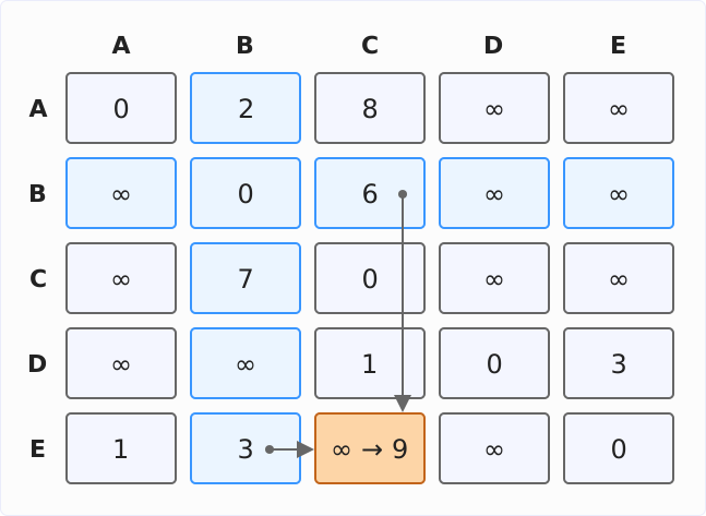
The following diagram shows this for iteration 2 of the example above, that is, for intermediate node B. Row B and column B are highlighted in blue, field (E, C) is orange: its new value 9 is the sum of row E, column B (3) and row B, column C (6). The arrows lead from these two fields to field (E, C). Field (A, C) already got its 8 earlier in this iteration:

The addCosts() method returns infinity (in the form of Integer.MAX_VALUE) if either of the two summands is infinity:

private static int addCosts(int a, int b) {
  if (a == Integer.MAX_VALUE || b == Integer.MAX_VALUE) {
    return Integer.MAX_VALUE;
  }
  return a + b;
}

Detecting Negative Cycles

After running through the iterations, we check for negative cycles:

for (int i = 0; i < n; i++) {
  if (m.costs[i][i] < 0) {
    throw new IllegalArgumentException("Graph has a negative cycle");
  }
}

In the end, the findShortestPaths() method returns the FloydWarshallMatrices instance m.

Determining the Shortest Path Between Two Nodes

I implemented the calculation of the shortest path from one node to another in the method FloydWarshallMatrices.getPath(). i and j are the indices of the start and end nodes:

if (successors[i][j] == -1) {
  return Optional.empty();
}

List<String> path = new ArrayList<>();
path.add(nodes[i]);

while (i != j) {
  i = successors[i][j];
  path.add(nodes[i]);
}

return Optional.of(List.copyOf(path));

First we check if successors[i][j] is equal to -1. If this is the case, no path from i to j exists, and the method returns an empty Optional.

Otherwise, we create a list path and fill it with the initial node, and then – one by one – with the successor nodes of the path. Finally, we return an unmodifiable copy of the list (“defensive copy”).

Invoking the findShortestPaths() Method

The following three examples in the repository show how to invoke the findShortestPaths() method:

• TestWithSampleGraph: In this test, we calculate the shortest paths in the example graph from this article.
• TestWithSampleGraphFromBellmanFord: This test determines the shortest paths in the example graph from the article about the Bellman-Ford algorithm.
• TestWithNegativeCycle: This test invokes the findShortestPaths() method on an example graph with a negative cycle (also from the Bellman-Ford article).

Floyd-Warshall Time Complexity

The time complexity of the Floyd-Warshall algorithm is easily determined. We have three nested loops, each counting n passes. In the innermost loop, we have a comparison that can be performed in constant time. The comparison is performed n × n × n times – or n³ times.

The time complexity of Floyd-Warshall is thus: O(n³)

The space complexity is O(n²): the cost matrix has n × n fields, and the optional successor matrix has as many again.

Floyd-Warshall Runtime

Using the program TestFloydWarshallRuntime, we can check whether the algorithm’s running time fits the inferred time complexity O(n³). The program creates random graphs of different sizes and calculates the shortest paths in them. It repeats each test 50 times and outputs the median of all measured values. I measured on an Apple M5 Pro with Java 27.

The following diagram shows the runtime as a function of the graph’s size:

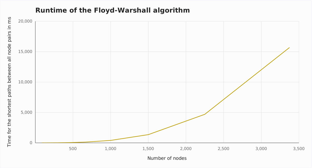
The cubic growth can be seen clearly. The measuring points are a factor of 1.5 apart, so the time should increase by a factor of 1.5³ ≈ 3.4 each time: from 1,000 to 1,500 nodes, it increases from 0.41 s to 1.35 s; at 2,250 nodes, it is 4.69 s, and at 3,375 nodes, 15.69 s. From 1,000 nodes on, that is 3.3 to 3.5 times as long from one step to the next.

Floyd-Warshall vs. Dijkstra vs. Bellman-Ford

In the following diagram, I compare the running times of Floyd-Warshall, Bellman-Ford (standard variant and optimized variant), and Dijkstra (with a Fibonacci heap). The Bellman-Ford values come from the article on the Bellman-Ford algorithm, measured on the same machine and on random graphs of the same kind. The Dijkstra values come from the article on Dijkstra’s algorithm – also from the same machine, but on graphs without negative edge weights, since Dijkstra cannot handle them. That measurement series starts at 10,000 nodes, which is why the Dijkstra line only begins there:

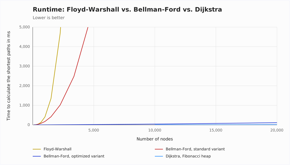
Floyd-Warshall is, as expected due to its time complexity, even slower than Bellman-Ford: at 2,250 nodes, Floyd-Warshall takes 4.7 s, the standard variant of Bellman-Ford 1.0 s.

To be fair, though: Floyd-Warshall calculates the paths between all pairs of nodes, while the other algorithms in the diagram only calculate the paths from a single start node. For all pairs, you would have to run Dijkstra n times. In a dense graph, where almost every node is connected to every other node, that also takes you to O(n³).

So when should which algorithm be used?

• Floyd-Warshall should only be used when the shortest paths between all node pairs are sought.
• Bellman-Ford should be used when the graph contains negative edge weights.
• A* should be used if the graph does not have negative edge weights and a heuristic can be defined.
• Without negative edge weights and without a heuristic, Dijkstra’s algorithm should be used.

Summary

This article has shown you when to use the Floyd-Warshall algorithm (when you need the shortest distances between all node pairs), how it works, and how it identifies negative cycles.

The time complexity of O(n³) is significantly worse than that of all pathfinding algorithms presented so far on sparse graphs – which, however, only calculate the paths from a single start node. Floyd-Warshall should, therefore, only be used for the intended purpose.

This concludes the series on pathfinding algorithms.